Unit 06 · Air, Atmosphere & Climate Change
Connect solar/atmospheric drivers to climate while distinguishing greenhouse forcing, ozone chemistry and air-pollutant exposure. Use budgets, matched-season trends, emissions trends, carbon-source comparisons and time-weighted concentrations without claiming a generated dataset proves attribution.
Student learning: Clean air, carbon sources, and testing climate explanations
Choose the level by readiness, not age alone, and record it before instruction. Foundation, core, and honors tasks are study pathways, not an AP course or a promise of college credit. The instructor retains practical assessment and the published science rubric; integration is reported separately.
Prerequisites: Units 3–5; energy budgets, time-weighted means, percent change, carbon-to-CO₂ mass conversion, concentration trends, and logarithms for the honors pH comparison.
Suggested sequence: read and discuss the explanation; attempt the worked model; analyze the data at your selected level; check the answers; then complete the source-linked response and a fresh transfer question. These activities supplement, not replace, supervised practical work and the full-year schedule.
Assigned reading and focus
- EPA: Air Quality – National Summary. Read Air Quality Trends and Emissions Trends, including the comparison of growth areas and emissions. Record the 1970–2025 changes EPA reports: gross domestic product +349%, vehicle miles traveled +197%, energy consumption +46%, population +67% and total emissions of the six principal air pollutants −78%. Note that about 115 million people still lived in counties above a primary air standard in 2025. Checked 2026-10-02.
- NASA: The Causes of Climate Change. Read Increasing Greenhouse Gases Are Warming the Planet, the forcing/feedback definitions, and Evidence Shows That Current Global Warming Cannot Be Explained by Solar Irradiance, including the Sun’s role in past changes such as the Little Ice Age. List evidence beyond a single temperature graph.
- CSIRO: Global Carbon Budget 2025 news release. Read the opening and Key findings. Record the projected 42.2 billion tonnes of CO₂ from all human activities in 2025, the fossil-fuel share of about 90 percent, and the past-decade shares absorbed by land (21 percent) and ocean (29 percent). Separate the reported findings from the policy recommendation quoted near the end. Checked 2026-10-02.
- USGS Volcano Hazards Program: Volcanoes Can Affect Climate. Read the section asking whether volcanoes emit more CO₂ than human activities and the yearly CO₂ emitters table. Record the published 0.13–0.44 billion tonne range for all volcanoes and the 0.26 highest preferred estimate. Checked 2026-10-02.
- NASA: New NASA Study Tallies Carbon Emissions From Massive Canadian Fires. Read the whole article. Record the estimate of about 640 million metric tons of carbon from the May–September 2023 fires, the comparison with Russia’s and Japan’s 2022 fossil-fuel emissions, the statement about regrowing forests, and the contributing factors USDA lists for larger fires. Checked 2026-10-02.
- NOAA: What Are El Niño and La Niña?. Read the normal-conditions introduction and El Niño/La Niña sections. Sketch trade winds, warm water and upwelling; explain that regional effects are tendencies, not identical forecasts everywhere.
- EPA: Particulate Matter (PM) Basics. Read What is PM, and how does it get into the air? and What are the harmful effects of PM? Distinguish directly emitted particles from secondary formation and concentration from dose.
- EPA: Ground-level Ozone Basics. Read What is good vs. bad ozone? and How does ground-level ozone form? Identify stratospheric protection versus NOx/VOC/sunlight formation near the surface.
- NOAA Ocean Acidification Program: What Is Ocean Acidification?. Read the introductory ocean-chemistry explanation and How ocean acidification differs from climate change. Explain why warming and changing carbonate chemistry are distinct processes with a common CO₂ driver.
- OpenStax University Physics Volume 1: 17.3 Sound Intensity. [noise-energy] Noise levels do not average arithmetically: Read the logarithmic decibel definition and intensity addition. Do the arithmetic silently; do not reproduce sound levels.
- NOAA Ocean Service: What is ocean noise?. [noise-energy] Noise levels do not average arithmetically: Read how human-generated noise can interfere with marine communication. Distinguish an acoustic exposure metric from a biological effect.
- EPA: Air Pollution Control Cost Manual. [control-mass] A lower concentration may be dilution, not removal: Consult the particulate-control and gas-control sections. Identify the pollutant and mechanism before treating a device as a universal pollution solution.
- EPA: What is Acid Rain?. [acid-deposition] Rain acidity needs amount as well as pH: Read wet and dry deposition and the roles of SO₂ and NOx. Explain why rain pH alone misses dry deposition and neutralized acid inputs.
- EPA: Ground-level Ozone Basics. [smog-regimes] Precursor reductions need a chemistry and meteorology context: Read how ground-level ozone forms from NOx and VOCs in sunlight and why transport/weather matter. Distinguish primary precursor emissions from secondary ozone.
- NOAA Coral Reef Watch: daily global 5-km Degree Heating Week product, version 3.1. [ocean-heat] Accumulated marine heat stress and ecosystem response: Read the 12-week accumulation description and probabilistic bleaching/mortality risk discussion. Separate a risk indicator from a measured outcome at a reef.
- NOAA Coral Reef Watch: Coral Bleaching HotSpot method. [ocean-heat] Accumulated marine heat stress and ecosystem response: Read the maximum monthly mean reference and the HotSpot threshold used for accumulation; distinguish climatological reference from the current weekly average.
Learn the science
Clean air is common ground. EPA reports that from 1970 to 2025 total emissions of the six principal air pollutants fell 78% while the economy, driving, energy use and population all grew, and it credits state and federal rules and technological advances for much of a separate decline in air toxics. Families still debate which rules are worth their costs, and the work is not finished: EPA estimates about 115 million people lived in counties above a primary air standard in 2025.
The troposphere contains most weather and usually cools with altitude; stratospheric ozone absorbs ultraviolet energy and helps produce warming with altitude there. Uneven solar heating and rotation help organize global wind patterns. An inversion can suppress vertical mixing near the surface, raising local pollutant concentrations without itself establishing a global climate trend.
For a top-of-atmosphere mean budget, net energy gain is incoming sunlight minus reflected sunlight minus outgoing infrared. Greenhouse gases absorb and re-emit infrared; they do not create energy. Persistent positive imbalance increases stored energy, but temperature response also depends on heat capacity, circulation and feedbacks.
CO₂ and methane can act as forcings when their abundance changes; water-vapor increase is an important warming feedback. Ranking gases requires a specified metric, abundance and time horizon. Climate also changes for natural reasons: NASA notes that lower solar activity and more volcanic activity helped trigger the Little Ice Age, and ENSO shifts heat from year to year. NASA tests those alternatives against the evidence and attributes modern warming mainly to human influence. Families disagree about how large the human share is and what policy should follow, and this unit takes no policy position. The synthetic graph here does not independently establish attribution.
Normal tropical Pacific trade winds push surface water west and permit eastern upwelling. El Niño weakens this pattern; La Niña strengthens it. ENSO redistributes heat and changes regional precipitation and ecosystems. It is not a substitute explanation for the long-term externally forced warming trend, nor a perfectly periodic clock.
A Keeling-type record can show both a multiyear rise and a seasonal cycle influenced by land-plant uptake and respiration. Compare the same season across years. Six deliberately generated points are not the actual Keeling record and do not support attribution, a complete carbon budget or an extrapolated climate sensitivity.
To test where added CO₂ comes from, compare candidate sources by size and by what happens to their carbon afterward. Convert a carbon mass to CO₂ by multiplying by 44/12. USGS puts all volcanoes at 0.13–0.44 billion tonnes of CO₂ a year, less than 1% of human emissions. Wildfires can be very large: NASA estimates the 2023 Canadian fires released about 640 million tonnes of carbon in five months, more than Russia or Japan emitted from fossil fuels in 2022. As forests regrow they reabsorb that carbon, while fossil-fuel CO₂ is not readily offset by natural processes. The Global Carbon Budget reports that over the past decade land and ocean absorbed about half of human emissions. If natural sources were driving the rise, the air would gain more CO₂ than people add, not about half as much.
Ground-level ozone is a secondary pollutant formed through NOx/VOC reactions in sunlight. Stratospheric ozone depletion involves ozone-depleting chemicals and UV chemistry; it is not the greenhouse mechanism. SO₂ and NOx can contribute to acid deposition. PM₂.₅ is defined by particle size, not one chemical composition; indoor and outdoor exposures can differ.
A time-weighted concentration uses sum(concentration × hours)/total hours. It is not inhaled dose unless breathing rates and uptake are also modeled, and it is not an AQI: AQI uses pollutant-specific averaging rules and breakpoints. Do not generate smoke, alter ventilation deliberately, or expose anyone to pollutants to obtain observations.
Wildfire smoke ties forests, climate and clean air together. EPA lists fires among the direct sources of fine particles, so smoke can raise PM₂.₅ exposure indoors and out. NASA cites USDA findings that the number, severity and size of wildfires have increased in recent decades, with contributing factors that include extended drought, past fire-management strategies, invasive species and homes built in formerly less developed areas. Forest management, fuel reduction and planning for smoky days are practical steps whatever one concludes about climate; each has costs and tradeoffs a community has to weigh.
Dissolving CO₂ changes seawater carbonate chemistry: more hydrogen ions reduce carbonate available to many shell-building organisms. A change from pH 8.2 to 8.1 means hydrogen-ion activity increases by 10^0.1, about 26%, while the water is still alkaline. This is not a 0.1% change. Biological responses depend on species and other conditions, and ocean warming is a separate stressor.
[noise-energy] Noise levels do not average arithmetically: Traffic, construction and industrial or vessel noise can interfere with communication and affect humans or wildlife, depending on frequency, duration and context. Decibels are logarithmic: a ten-decibel rise is ten times the corresponding intensity, not ten percent. Equivalent level Leq = 10 log10[sum(t×10^(L/10))/sum(t)] for compatible time intervals and weighting. A-weighted air levels and underwater sound levels use different conventions and reference pressures and must not be directly compared.
[noise-energy] Noise levels do not average arithmetically: Model and provenance assumptions: The synthetic air records are compatible A-weighted levels at one receptor, constant within three hours and one hour. The additional two-source example assumes incoherent equal sources with the same geometry. Calculations are silent; no noise generation or exposure measurement is assigned.
[noise-energy] Noise levels do not average arithmetically: Uncertainty and inference limits: Leq hides short peaks and frequency content. It is not an exposure limit, clinical assessment or proof of ecological harm. These air calculations cannot be applied numerically to the linked underwater examples without changing reference, medium and weighting.
[control-mass] A lower concentration may be dilution, not removal: Fabric filters and electrostatic precipitators capture particles, while sulfur-gas scrubbers or NOx reduction systems address different chemical pathways. Captured material may become a residue needing management; it does not disappear. Removal efficiency should compare inlet and outlet mass rates under compatible gas-volume conventions. Dilution can lower concentration without lowering mass discharge. Bypass time can reduce shift-wide performance even when the operating device works well.
[control-mass] A lower concentration may be dilution, not removal: Model and provenance assumptions: Synthetic PM inlet/outlet concentrations use the same dry standard-volume basis; outlet flow is larger because of added clean gas. Flow and concentration are fixed within each interval. The device runs seven hours and bypasses one, with no other particle source or storage change.
[control-mass] A lower concentration may be dilution, not removal: Uncertainty and inference limits: With outlet concentration 8–12 instead of 10 mg/m³ and fixed flows, operating removal ranges 90.4–85.6%. Instrument bias, flow normalization and bypass logs need review. No stack, roadside or hazardous air sampling is assigned.
[acid-deposition] Rain acidity needs amount as well as pH: Atmospheric transformation of SO₂ and nitrogen oxides can contribute to sulfuric and nitric acids transported and deposited away from sources. Wet deposition carries dissolved material; dry deposition occurs without precipitation. pH describes hydrogen-ion activity, not total acid delivered. For this dilute unbuffered model only, approximate [H⁺] = 10^(−pH) mol/L and multiply by rain volume per area. Buffered soils or waters can consume hydrogen ions, so free-H⁺ load is not total acidity or ecological damage.
[acid-deposition] Rain acidity needs amount as well as pH: Model and provenance assumptions: Two synthetic storms reach one square meter. One mm rain equals one liter/m². Use common temperature, ideal dilute concentrations and no reactions during mixing. The model does not include sulfate/nitrate speciation, alkalinity or dry deposition.
[acid-deposition] Rain acidity needs amount as well as pH: Uncertainty and inference limits: Measurement on a logarithmic scale means pH ±0.1 changes modeled H⁺ by factors 10^∓0.1, not by ±0.1%. Carbonate reactions and ionic activity can invalidate the simple mixture estimate. No collection or acid-handling procedure is assigned.
[smog-regimes] Precursor reductions need a chemistry and meteorology context: Photochemical smog includes secondary pollutants formed in reactions involving nitrogen oxides, volatile organic compounds and sunlight. Ozone is not directly emitted in the same way as many precursors. NO can remove local ozone by titration, while NO₂ photochemistry and peroxy radicals can support net production. In a VOC-limited setting, a NOx reduction can raise a local peak; in a NOx-limited setting it can lower it. The response depends on chemistry, transport and meteorology, not one universal percentage rule.
[smog-regimes] Precursor reductions need a chemistry and meteorology context: Model and provenance assumptions: These synthetic response cards stipulate two chemistry regimes, with weather and sunlight held fixed within each paired comparison. NOx and VOC values are scenario inputs, not measurements or a mechanistic chemical model fitted here. Ozone is the modeled maximum one-hour concentration in ppb.
[smog-regimes] Precursor reductions need a chemistry and meteorology context: Uncertainty and inference limits: Different weather, mixing and precursor mixtures can reverse or weaken a response. A modeled one-hour peak is not regulatory attainment or an eight-hour standard comparison. These cards illustrate a hypothesis to test with vetted records, not instructions to produce smog or sample polluted air.
[ocean-heat] Accumulated marine heat stress and ecosystem response: Ocean warming changes stratification, oxygen solubility, habitat ranges and marine heatwaves; it is not identical to acidification. Corals can lose symbiotic algae under sustained heat stress, but bleaching is not always immediate death. NOAA’s Degree Heating Week method accumulates HotSpots at least 1 °C above a local maximum monthly mean over the preceding twelve weeks. Here constant-within-week records make daily accumulation divided by seven equivalent to summing qualifying degree-weeks.
[ocean-heat] Accumulated marine heat stress and ecosystem response: Model and provenance assumptions: All four synthetic weeks last seven days; the previous eight weeks in the twelve-week window have zero qualifying stress. Maximum monthly mean is fixed at 28 °C. Cover records use the same recognition method one year apart, but are not randomized exposure treatments.
[ocean-heat] Accumulated marine heat stress and ecosystem response: Uncertainty and inference limits: SST error ±0.2 °C can switch a week across the 1 °C inclusion threshold: this window ranges 3.1–5.1 °C-weeks. Cover change can reflect storms, disease or sampling as well as heat. The indicator is not a NOAA observation and does not itself measure bleaching, mortality or attribution.

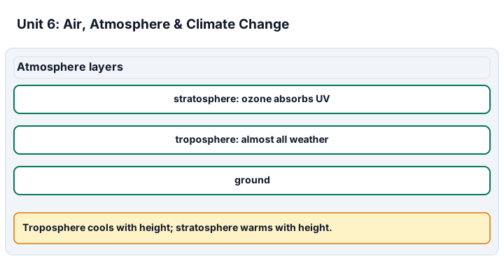
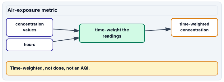
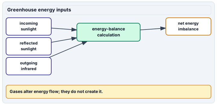
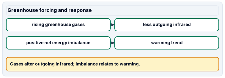
Diagram description
The atmosphere panel lists the stratosphere, where ozone absorbs ultraviolet energy and air warms with height, above the troposphere, where almost all weather happens and air usually cools with height, above the ground, with no arrows between layers. Exposure is a time-weighted concentration, not dose or AQI. Greenhouse energy panels combine incoming sunlight, reflected sunlight and outgoing infrared; rising greenhouse gases reduce outgoing infrared, and a positive net energy imbalance relates to a warming trend.
Data, provenance, and assumptions
| Incoming solar (W/m²) | Reflected solar (W/m²) | Outgoing infrared (W/m²) |
|---|---|---|
| 340 | 102 | 237 |
| Year index | Month | CO₂ (ppm) |
|---|---|---|
| 0 | May | 410 |
| 0 | September | 405 |
| 1 | May | 412 |
| 1 | September | 407 |
| 2 | May | 414 |
| 2 | September | 409 |
| Location | Duration (hours) | PM₂.₅ (µg/m³) |
|---|---|---|
| Indoors | 16 | 25 |
| Outdoors | 8 | 10 |
| Initial pH | Later pH |
|---|---|
| 8.2 | 8.1 |
| Measure, 1970 to 2025 | Reported change (%) |
|---|---|
| Gross domestic product | 349 |
| Vehicle miles traveled | 197 |
| Energy consumption | 46 |
| Population | 67 |
| Total emissions of the six principal air pollutants | -78 |
| Source or sink | Reported value | Unit |
|---|---|---|
| All human activities, 2025 projection | 42.2 | billion tonnes CO₂ per year |
| Fossil-fuel share of human emissions | 90 | percent, approximate |
| Land uptake, past-decade average | 21 | percent of human emissions |
| Ocean uptake, past-decade average | 29 | percent of human emissions |
| All volcanoes, highest preferred estimate | 0.26 | billion tonnes CO₂ per year |
| 2023 Canadian wildfires, May–September | 640 | million tonnes of carbon |
| Interval | Duration (hours) | Equivalent air level (dBA) |
|---|---|---|
| Background period | 3 | 60 |
| Construction model period | 1 | 70 |
| Inlet (mg/m³) | Inlet flow (m³/hour) | Controlled outlet (mg/m³) | Outlet flow (m³/hour) | Controlled hours | Bypass hours |
|---|---|---|---|---|---|
| 100 | 1000 | 10 | 1200 | 7 | 1 |
| Storm | Rain volume (L/m²) | pH |
|---|---|---|
| A | 10 | 4 |
| B | 100 | 5 |
| Regime / control | NOx input (ppb) | VOC input (ppbC) | Peak one-hour ozone (ppb) |
|---|---|---|---|
| Urban VOC-limited baseline | 40 | 100 | 80 |
| Urban NOx reduction | 20 | 100 | 90 |
| Rural NOx-limited baseline | 40 | 200 | 80 |
| Rural NOx reduction | 20 | 200 | 50 |
| Week in window | Duration (weeks) | SST (°C) | Maximum monthly mean (°C) |
|---|---|---|---|
| 9 | 1 | 29 | 28 |
| 10 | 1 | 30 | 28 |
| 11 | 1 | 28.5 | 28 |
| 12 | 1 | 29.5 | 28 |
| Site | Before cover (%) | After cover (%) |
|---|---|---|
| Warm site | 40 | 30 |
| Refuge site | 40 | 38 |
Worked model
The energy imbalance is 340 − 102 − 237 = +1 W/m², with 30% reflected. Matched May CO₂ increases (414 − 410)/2 = 2 ppm/year despite each seasonal decline. Time-weighted PM₂.₅ = (25 × 16 + 10 × 8)/24 = 20 µg/m³, not the unweighted 17.5. The pH ratio is 10^(8.2 − 8.1) ≈ 1.258925. Converting fire carbon to CO₂: 640 × 44/12 ≈ 2,347 million tonnes, or about 2.35 billion tonnes of CO₂. [noise-energy] Noise levels do not average arithmetically: Leq = 10 log10[(3×10⁶ + 1×10⁷)/4] ≈ 65.118834 dBA, not the arithmetic 62.5. Two equal incoherent 60-dBA sources at the receptor combine to 60 + 10 log10(2) ≈ 63.010300 dBA, not 120 dBA. [control-mass] A lower concentration may be dilution, not removal: Inlet mass = 100×1000/1000 = 100 g/hour; outlet = 10×1200/1000 = 12 g/hour. Operating removal is 88%, not the 90% concentration reduction. Shift emissions = 7×12 + 1×100 = 184 g; captured residue = 7×88 = 616 g. Together they equal the 800-g inlet, giving 77% shift removal. [acid-deposition] Rain acidity needs amount as well as pH: Storm A contributes 10×10⁻⁴ = 0.001 mol H⁺/m²; B contributes 100×10⁻⁵ = 0.001 too. Total is 2 mmol/m². Mixing without reaction gives concentration 0.002/110 mol/L and pH ≈ 4.740363, not the arithmetic mean 4.5. [smog-regimes] Precursor reductions need a chemistry and meteorology context: Urban NOx reduction changes ozone (90−80)/80 ×100 = +12.5%; rural reduction changes it (50−80)/80 ×100 = −37.5%. Both halve the NOx input, yet ozone responds differently. A claim that cutting a precursor by half must cut ozone by half is unsupported. [ocean-heat] Accumulated marine heat stress and ecosystem response: HotSpots are 1, 2, 0.5 and 1.5 °C. Only those at least one contribute: 1 + 2 + 0 + 1.5 = 4.5 °C-weeks. Warm-site cover falls 10 percentage points, or 10/40 × 100 = 25% relative to its starting cover. A comparison-site difference is not causal attribution.
Numerical calibration
- 1 W/m²
- 30 %
- 2 ppm/year
- 20 µg/m³
- 11.333333 µg/m³
- 1.258925 dimensionless activity ratio
- -95.100223 % change in total emissions per dollar of GDP, 1970–2025
- -86.826347 % change in total emissions per person, 1970–2025
- 2.346667 billion tonnes CO₂ from the 2023 Canadian fires
- 5.560821 % of 2025 human CO₂ emissions
- 0.616114 % of 2025 human CO₂ emissions
- 21.1 billion tonnes CO₂ staying in the air under past-decade sink shares
- 65.1188336098 dBA over four modeled hours
- 63.0102999566 dBA for two equal incoherent sources
- 68.8930170251 dBA over four modeled hours
- 88 % operating mass removal
- 184 g PM/eight-hour shift
- 616 g captured PM/eight-hour shift
- 77 % shift mass removal
- 85.6 % removal at outlet concentration 12 mg/m³
- 90.4 % removal at outlet concentration 8 mg/m³
- 76 % operating mass removal
- 2 mmol modeled free H⁺/m² across two events
- 4.7403626895 pH under ideal no-reaction mixing
- 0.7943282347 H⁺ multiplier for pH 0.1 higher
- 1.2589254118 H⁺ multiplier for pH 0.1 lower
- 2.2 mmol modeled free H⁺/m² across two events
- 12.5 % of baseline one-hour ozone
- -37.5 % of baseline one-hour ozone
- -35 % of baseline one-hour ozone
- 4.5 °C-weeks over preceding twelve weeks
- 25 % of starting cover lost
- 3.1 °C-weeks with all SST inputs 0.2 °C lower
- 5.1 °C-weeks with all SST inputs 0.2 °C higher
- 5.2 °C-weeks over preceding twelve weeks
Attempt the assigned level
Try the tasks before reading the calibration. These are practice answers, not a secure examination; use a new dataset or changed assumption for the assessed transfer.
Foundation
- Calculate the energy imbalance and label shortwave input, reflection and outgoing infrared.
- Plot all CO₂ points and compare May-to-May versus May-to-September differences. Match ozone, particles and greenhouse gases to their distinct mechanisms.
- Use the EPA table to state what happened to total emissions of the six principal pollutants while GDP, driving, energy use and population grew from 1970 to 2025, and what fraction of the 1970 emissions remained in 2025.
- [noise-energy] Noise levels do not average arithmetically: Explain the intensity ratio represented by 70 versus 60 dBA and calculate the time-weighted intensity before converting back to decibels.
- [control-mass] A lower concentration may be dilution, not removal: Calculate inlet and outlet mass rates and compare concentration reduction with mass removal. Explain the role of the changed outlet flow.
- [acid-deposition] Rain acidity needs amount as well as pH: Convert each pH to the modeled hydrogen-ion concentration and then to amount per area. Which storm delivers more free H⁺?
- [smog-regimes] Precursor reductions need a chemistry and meteorology context: Calculate ozone percent change for both paired NOx reductions and distinguish the precursor input from the secondary-pollutant response.
- [ocean-heat] Accumulated marine heat stress and ecosystem response: Calculate the qualifying heat accumulation and warm-site absolute and relative cover change. Explain why the 0.5 °C week is not included in this indicator.
Check after your attempt
- The imbalance is +1 W/m² and reflected fraction 0.30. Energy is accumulating under this idealized fixed budget.
- May values rise 2 ppm each year while each May-to-September decline is 5 ppm. A seasonal decrease is compatible with an underlying rise; ozone depletion, particle exposure and infrared absorption are different mechanisms.
- Emissions fell 78%, so 22% of the 1970 amount remained, while GDP grew 349%, driving 197%, energy use 46% and population 67%. In this record cleaner air did not require a shrinking economy; the table alone does not show which rule or technology caused which part of the decline.
- [noise-energy] Noise levels do not average arithmetically: The modeled corresponding intensity ratio is ten. Weighted intensity relative to the common reference is 3250000, giving about 65.118834 dBA; averaging the decibel labels loses the logarithmic scale.
- [control-mass] A lower concentration may be dilution, not removal: Mass rates are 100 and 12 g/hour; concentration falls 90% while mass falls 88%. Added clean gas changes volume, so the concentration ratio alone overstates capture.
- [acid-deposition] Rain acidity needs amount as well as pH: Concentrations are 0.0001 and 0.00001 mol/L, but both deliver 0.001 mol/m² because B has ten times the volume. The lower pH does not automatically mean the larger deposited amount.
- [smog-regimes] Precursor reductions need a chemistry and meteorology context: Urban change is +12.5% and rural −37.5%; neither equals the 50% NOx decrease. Ozone is a secondary product affected by reaction pathways, not the same measured quantity as precursor input.
- [ocean-heat] Accumulated marine heat stress and ecosystem response: Accumulation is 4.5 °C-weeks; cover change is −10 percentage points or a 25% relative loss. The 0.5 °C HotSpot is below the stipulated 1 °C accumulation threshold, although it is still warmer than the reference.
High-school core: typically grades 9-10
- Calculate the time-weighted PM mean and the revised mean when only indoor concentration becomes 12.
- Explain what ENSO redistributes and why this short synthetic CO₂ sequence cannot attribute warming to a cause.
- Convert the 2023 Canadian wildfire carbon to CO₂ and express it and the volcanic estimate as percentages of 2025 human emissions. Explain why fire CO₂ and fossil-fuel CO₂ act the same way once in the air but differ over decades.
- [noise-energy] Noise levels do not average arithmetically: Calculate the combined level of two equal incoherent 60-dBA sources and identify why this does not justify a claim about hearing safety or fish response.
- [control-mass] A lower concentration may be dilution, not removal: Include the bypass hour in shift emissions, capture and removal efficiency. Identify where the removed particle mass goes.
- [acid-deposition] Rain acidity needs amount as well as pH: Calculate combined free-H⁺ load and ideal mixture pH, then identify two acid-deposition inputs omitted by this calculation.
- [smog-regimes] Precursor reductions need a chemistry and meteorology context: Explain the roles of sunlight, VOC limitation and NO titration, and state why the two rows do not establish a universal control strategy.
- [ocean-heat] Accumulated marine heat stress and ecosystem response: Connect heat stress to two ecosystem mechanisms and distinguish them from acidification. Does the cover table prove heat caused the observed-in-the-model decline?
Check after your attempt
- The means are 20 and about 11.333 µg/m³. Neither is a dose, AQI or safety verdict.
- ENSO changes ocean–atmosphere heat distribution and circulation. Attribution needs independent physical and observational evidence; consult NASA’s evidence rather than treating generated points as proof.
- 640 million tonnes of carbon × 44/12 ≈ 2.35 billion tonnes of CO₂, about 5.6% of 42.2; volcanoes at 0.26 are about 0.6%. Once in the air both trap heat the same way, but regrowing forests reabsorb fire carbon over time, while fossil-fuel CO₂ is not readily offset. One extreme season in one country is not the global yearly fire total, and NASA notes that more frequent fires could offset some of the forests’ uptake.
- [noise-energy] Noise levels do not average arithmetically: The combined level is about 63.010300 dBA. Duration, frequency, receptor and biological context matter; air A-weighting is not an underwater convention and this calculation is not health guidance.
- [control-mass] A lower concentration may be dilution, not removal: Emissions total 184 g and captured mass 616 g from 800 g entering: 77% removal over the shift. Captured particles enter a residue stream; controls can transfer a burden to waste handling.
- [acid-deposition] Rain acidity needs amount as well as pH: Load is 2 mmol/m² and ideal mixture pH about 4.740363. Dry deposition and acid already neutralized by buffering are omitted; sulfate/nitrate and alkalinity records are needed for a fuller budget.
- [smog-regimes] Precursor reductions need a chemistry and meteorology context: Sunlight drives photochemistry; VOC availability constrains radical pathways, and lower NO can reduce local ozone removal. Regime, meteorology and transport determine response, so these synthetic examples require site-specific validation before control decisions.
- [ocean-heat] Accumulated marine heat stress and ecosystem response: Heat can disturb coral–algal symbiosis and strengthen stratification or reduce oxygen solubility. Acidification changes carbonate chemistry. The synthetic cover contrast has other possible drivers and does not establish a unique cause.
Honors extension: typically grades 11-12
- Compute the hydrogen-ion ratio for the paired pH values, and explain what remains unknown about a particular organism.
- Increase reflected solar by 3 W/m² while initially holding the other budget terms fixed. Calculate the new imbalance and identify why this is not a final equilibrium prediction.
- Using the carbon-budget shares, estimate how much of the 42.2 billion tonnes stayed in the air. Explain what this mass balance shows about whether natural sources, including fires and volcanoes, could be driving the long-term CO₂ rise.
- Find the percent change from 1970 to 2025 in total emissions per dollar of GDP and per person. What can and can’t this national trend tell you about one town’s air?
- [noise-energy] Noise levels do not average arithmetically: Propose a supplied-record comparison of a noise-control barrier, keeping receptor position, traffic and time consistent, with no actual exposure exercise.
- [control-mass] A lower concentration may be dilution, not removal: Bound operating removal for outlet concentration 8–12 mg/m³. What matched records would distinguish poor capture from a flow-normalization error?
- [acid-deposition] Rain acidity needs amount as well as pH: Explain how ±0.1 pH uncertainty propagates and why equal free-H⁺ load need not have equal ecological effect on two different catchments.
- [smog-regimes] Precursor reductions need a chemistry and meteorology context: Propose a safe supplied-record study comparing NOx-only, VOC-only and combined control under matched meteorology, with a declared averaging period.
- [ocean-heat] Accumulated marine heat stress and ecosystem response: Apply ±0.2 °C SST bounds to every week and recalculate the indicator. Propose independent records needed to test a heat–cover mechanism.
Check after your attempt
- The ratio is about 1.258925, a 25.89% increase on the stated scale; both values remain above 7. Species response also depends on carbonate saturation, acclimation and other stressors.
- The initial imbalance becomes −2 W/m². Temperatures, water vapor, clouds and outgoing radiation may adjust; a fixed-term perturbation is not a complete climate model.
- Land took about 21% and ocean about 29%, so about 50%, roughly 21.1 billion tonnes, stayed in the air; applying past-decade shares to one year is an approximation. Because the air gained less CO₂ than people added, land and ocean together, fires and volcanoes included, removed more than they released. Natural events still swing single years: the Global Carbon Budget reports weaker natural sinks in 2024 during El Niño, and a fire season like Canada’s 2023 adds a large pulse. Neither explains the long-term rise.
- Per dollar of GDP: 0.22/4.49 − 1 ≈ −95.1%. Per person: 0.22/1.67 − 1 ≈ −86.8%. The trend is national and combines six pollutants; one town’s air depends on its own sources, weather, terrain and monitors, and EPA still counts about 115 million people in counties above a primary standard.
- [noise-energy] Noise levels do not average arithmetically: Compare matched source-operation intervals and fixed receptor geometry before/after, retain frequency/peak information and repeated independent periods. Traffic changes could mimic barrier performance; paper records avoid hazardous monitoring.
- [control-mass] A lower concentration may be dilution, not removal: Removal ranges 90.4% down to 85.6%. Need synchronized inlet/outlet concentration, standard dry gas flows, particle definition, instrument checks and bypass records; concentration alone cannot diagnose capture failure.
- [acid-deposition] Rain acidity needs amount as well as pH: H⁺ scales by about 0.7943 to 1.2589 times the central value. Buffer capacity, soil chemistry, sensitive organisms and exposure timing differ; free-H⁺ arithmetic is not total acidity or proof of ecosystem harm.
- [smog-regimes] Precursor reductions need a chemistry and meteorology context: Use vetted chemistry simulations or existing paired monitoring records with fixed one-hour or eight-hour definitions, repeated periods and weather covariates. Distinguish a modeled response from causal field proof and from regulatory compliance.
- [ocean-heat] Accumulated marine heat stress and ecosystem response: The lower combination gives 0 + 1.8 + 0 + 1.3 = 3.1; the upper gives 1.2 + 2.2 + 0 + 1.7 = 5.1 °C-weeks. Seek repeated cover/bleaching, storm, disease and local temperature records; the threshold makes propagation nonlinear.
History, reading, and writing connection
Compare NOAA’s history of observations of warm Pacific waters with NASA’s climate evidence and the carbon-source readings. Write how an observed pattern becomes a testable mechanism, which natural explanations (ENSO, the Sun, volcanoes and wildfires) each source tests, and what the evidence shows about each. Close with one clean-air or forest-stewardship step your community could measure, its cost and who decides, keeping that policy view separate from the science.
Write in your own words or use an approved accessible equivalent. Cite a specific assigned section or figure, identify its evidence, and state one limitation or counterargument. Use the AI practice contract only for permitted coaching, never to invent observations or write the assessed response.
Transfer to a new case
A new synthetic air record has 40 µg/m³ for six hours and 10 µg/m³ for eighteen. What is the time-weighted mean, and can it be called inhaled dose? [noise-energy] Noise levels do not average arithmetically: A fresh silent model reverses the schedule: three hours at 70 dBA and one at 60 dBA at the same receptor. Calculate Leq without assuming the earlier answer still applies. [control-mass] A lower concentration may be dilution, not removal: A fresh dilution scenario retains inlet 100 mg/m³ at 1000 m³/hour and outlet 10 mg/m³, but outlet flow becomes 2400 m³/hour. Find operating mass-removal efficiency. [acid-deposition] Rain acidity needs amount as well as pH: A fresh pair of synthetic storms each delivers 20 L/m², at pH 4 and pH 5 under the same ideal assumptions. Find total free-H⁺ load in mmol/m², not an average pH. [smog-regimes] Precursor reductions need a chemistry and meteorology context: A fresh vetted-model exercise for another airshed gives one-hour ozone 60 ppb before and 39 ppb after a combined precursor change, with weather fixed. Find percent change; can it validate the urban NOx-only policy? [ocean-heat] Accumulated marine heat stress and ecosystem response: A fresh twelve-week synthetic window has eight zero-stress weeks and four one-week HotSpots of 1.2, 0.8, 2 and 2 °C. Compute the same heat indicator and state why it is not a guaranteed death count.
Calibration: The mean is (40 × 6 + 10 × 18)/24 = 17.5 µg/m³. It is not dose; breathing volume, uptake and other exposures have not been specified. [noise-energy] Noise levels do not average arithmetically: Leq = 10 log10[(3×10⁷ + 10⁶)/4] ≈ 68.893017 dBA. More time at the higher intensity raises the equivalent level; it remains a model, not an exposure recommendation. [control-mass] A lower concentration may be dilution, not removal: Outlet mass is 24 g/hour against 100 entering, so removal is 76%. The unchanged concentration reduction still does not establish unchanged mass control. [acid-deposition] Rain acidity needs amount as well as pH: Load is (20×10⁻⁴ + 20×10⁻⁵)×1000 = 2.2 mmol/m². Equal volumes now make the lower-pH storm deliver ten times the free-H⁺ amount. [smog-regimes] Precursor reductions need a chemistry and meteorology context: Change is (39−60)/60 ×100 = −35%. It concerns another regime and a combined intervention, so it does not validate a NOx-only strategy for the earlier urban setting. [ocean-heat] Accumulated marine heat stress and ecosystem response: The qualifying sum is 1.2 + 0 + 2 + 2 = 5.2 °C-weeks. Organism sensitivity, acclimation and other stressors vary; the risk indicator is not a count or a guarantee of mortality.
Evidence to retain
Keep the budget, matched-season plot, exposure calculation, emissions-trend and carbon-source calculations, and source-based mechanism distinctions. State sample duration and uncertainty, and label simulations rather than presenting them as personal air monitoring. [noise-energy] Noise levels do not average arithmetically: Retain the logarithmic/time-weighted calculation, compatible-reference note and matched-control design. Use Unit 6 pollution, controls and data criteria; supplied acoustic numbers do not certify a safe exposure or performed monitoring. [control-mass] A lower concentration may be dilution, not removal: Retain matched gas-volume units, inlet/outlet and bypass mass balance, residual-waste note and uncertainty bounds. Use Unit 6 pollutant/control/data criteria; no control equipment or hazardous emissions testing is performed. [acid-deposition] Rain acidity needs amount as well as pH: Retain concentration-to-area conversions, the non-arithmetic pH mixture, wet/dry deposition mechanism and buffering limits. Use Unit 6 pollution, control and data criteria; supplied storm values are not a hazardous sampling assignment. [smog-regimes] Precursor reductions need a chemistry and meteorology context: Retain paired precursor/ozone contrasts, a nonlinear-chemistry explanation and a matched-period study proposal. Use Unit 6 pollutant, control and data criteria; a lower model concentration is not proof of compliance or safe air. [ocean-heat] Accumulated marine heat stress and ecosystem response: Retain the thresholded twelve-week heat calculation, cover denominators, SST sensitivity bounds and a warming-versus-acidification mechanism diagram. Use Unit 6 radiation/climate/data criteria; an inland supplied-record alternative is the default.
Record units, calculations, source/date, uncertainty, and what is measured versus inferred. A simulation or supplied dataset must stay labeled as such. Use supplied data or an instructor-approved supervised observation. No electrical work, combustion, radioactive materials, pesticide application, wildlife capture, microbial culture, hazardous sampling or sample ingestion is authorized.
Return to all eight learning pathways. Print this unit page for the student lessons; the linked five-page packet remains the separate assessment companion.
Unit mastery rubric
| Criterion | Developing | Proficient | Mastery |
|---|---|---|---|
| Atmospheric structure and circulation | Treats all layers as identical. | Names layers without mechanisms. | Explains troposphere/stratosphere differences, solar/rotation-driven circulation, inversions and ENSO-related redistribution. |
| Radiation balance and climate mechanisms | Confuses ozone with greenhouse warming. | Names gases without a budget. | Calculates an energy imbalance; distinguishes forcing from feedback and states the metric needed to compare greenhouse gases. |
| Carbon records and attribution | Confuses seasonal change and trend. | Plots values with help. | Calculates matched-season change, relates carbon uptake/emissions to a record, and uses independent evidence for attribution. |
| Ozone, deposition, particles and noise | Conflates air-pollution mechanisms. | Names pollutants without pathways. | Distinguishes smog, deposition, PM and noise; computes time/intensity weighting and control mass balances without claiming dose, AQI or safety. |
| Environmental data technique | Omits metadata or invents monitoring. | Calculates without limits. | Defends an approved air/climate dataset analysis with units, timing, uncertainty and a fresh transfer; separates observation from model. |
| Integration (cross-domain) | Makes no supported connection between the source and the science. | Uses the source but needs help connecting evidence, writing, or limitations to the science. | Independently connects History, Reading, and Writing using a cited source, appropriate evidence, a limitation, and a scientific explanation. |
Integration is reported separately and cannot lower the science grade or block a science demonstration pass. Science and practical criteria determine that pass. Use the integration guide's evidence checklist for the separately reported criterion.
The synthetic May values rise 2 ppm/year while each summer value falls. That is compatible with a seasonal cycle and trend, but attribution needs NASA’s independent evidence, not these six invented points.
CO₂ fell between May and September, so a longer-term rise is impossible.
Assess metadata, calculations and a mechanism-based defense. Do not ask learners to create smoke, enter unhealthy air or manipulate ventilation to collect data.
A 5-page clipboard packet — unit overview, key terms, the mastery rubric, anchor examples, and a score sheet you can print and grade against.