Unit 07 · Ocean Ecosystems
Reefs, estuaries, kelp forests, the open ocean and deep habitats differ in light, nutrients, salinity, oxygen and physical structure. Much of the deep seafloor depends on sinking organic matter; vents and seeps add localized chemosynthetic production. Not all deep-sea food webs are vent webs, and absence of sunlight does not mean absence of life.
Student learning: Compare communities with honest sampling and energy budgets
Choose the level by readiness, not age alone, and record it before instruction. Foundation, core, and honors tasks are study pathways, not an AP course or a promise of college credit. The instructor retains practical assessment and the published science rubric; integration is reported separately.
Prerequisites: Units 1–6 habitat, microbial loop, life stages and adaptations; area, pooled proportions and square terms.
Suggested sequence: read and discuss the explanation; attempt the worked model; analyze the data at your selected level; check the answers; then complete the source-linked response and a fresh transfer question. These activities supplement, not replace, supervised practical work and the full-year schedule.
Assigned reading and focus
- NOAA Ocean Exploration: Photosynthesis and Chemosynthesis. Read the opening contrast and the paragraph on the 1977 discovery of vent communities. Explain chemical energy for carbon fixation, while noting many organisms still need oxygen supplied from elsewhere. Use the prose comparison; do not reproduce the page’s unbalanced shorthand photosynthesis equation.
- NOAA National Marine Sanctuaries: Seagrass Meadows. Read the nursery, sediment and threats sections. Separate the habitat mechanisms from evidence that a particular site has more species or higher recruitment.
- NOAA: What is coral bleaching?. Read the opening paragraphs and infographic transcript; distinguish symbiont loss, stress and death. Use it to compare reef interactions with the supplied meadow/edge community model.
Learn the science
Reefs, estuaries, kelp forests, the open ocean and deep habitats differ in light, nutrients, salinity, oxygen and physical structure. Much of the deep seafloor depends on sinking organic matter; vents and seeps add localized chemosynthetic production. Not all deep-sea food webs are vent webs, and absence of sunlight does not mean absence of life.
Chemosynthetic microbes obtain energy from chemical reactions and fix inorganic carbon. For example, sulfide oxidation can support production where vent fluid meets oxidant-bearing seawater. Many vent animals still use oxygen ultimately linked to surface production and circulation; “independent of local sunlight” does not imply independent of every surface process.
Food-web arrows track transfer from resource to consumer. Primary producers respire, consumers respire, and the microbial loop processes dissolved organic matter. NPP = GPP − producer respiration. Grazer production/NPP is a carbon-transfer fraction only under a defined boundary and interval; no universal 10% rule is imposed.
The supplied A/B/C labels are operational morphotypes, not verified species. Richness counts represented types; Simpson diversity here is D = 1 − sum(p_i^2) using pooled counts. Equal richness or total abundance can accompany different dominance. This is the descriptive proportional form, not the sample-corrected estimator.
Defined area, nonoverlapping plots, equal effort and a prespecified inclusion rule make samples comparable. Points within plots and repeat readings are not independent site replicates. Detection, habitat coverage and identification error remain; a zero observation is not proof of absence.
Juvenile recruitment, predation, competition and mutualism can alter community structure. A reef coral’s photosynthetic partnership differs from a grazer consuming algae. Covarying temperature, salinity and oxygen prevent the meadow/edge comparison from isolating a single cause.

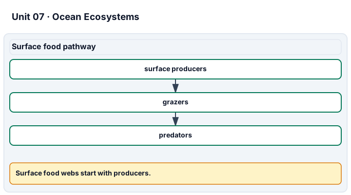
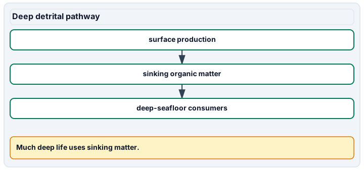
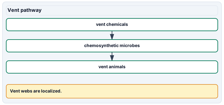
Diagram description
Surface producers feed grazers and predators. Some surface production becomes sinking organic matter that supports deep-seafloor consumers. Vent chemicals can power chemosynthetic microbes, which support vent animals. The vent path is separate from sinking detritus.
Data, provenance, and assumptions
| Habitat | Plot ID | Area (m^2) | A (grazer type) | B (filter-feeder type) | C (predator type) |
|---|---|---|---|---|---|
| Meadow | M1 | 0.25 | 4 | 4 | 2 |
| Meadow | M2 | 0.25 | 5 | 3 | 2 |
| Meadow | M3 | 0.25 | 3 | 5 | 2 |
| Edge | E1 | 0.25 | 8 | 1 | 1 |
| Edge | E2 | 0.25 | 9 | 1 | 0 |
| Edge | E3 | 0.25 | 7 | 2 | 1 |
| Habitat | Temperature (degrees C) | Practical Salinity | Oxygen (mg/L) |
|---|---|---|---|
| Meadow | 18 | 28 | 6.5 |
| Edge | 22 | 15 | 3 |
| Gross primary production | Producer respiration | Grazer production | Grazer respiration | Ungrazed/other NPP |
|---|---|---|---|---|
| 500 | 200 | 45 | 150 | 105 |
Complete inland analysis with an optional bounded observational comparison
Scope and safety: Instructor and site approval are required for any optional observation. Stay on a dry, accessible designated public viewing path or approved indoor viewing area; no wading, shore scrambling, tidal exposure, entering water, boat use, touching animals/plants, sampling or new plot installation. Cancel if conditions or visibility are unsuitable. Supplied analysis is not a field/practical credential.
Materials and preparation
- The three supplied tables, paper or an accessible spreadsheet, and the assigned NOAA readings
- Optional only: instructor-approved existing images or visible fixed plots with documented area and permission; no new field equipment deployment
- Record sheet with anonymous plot codes, time block, method, area/effort, counts/unknowns, provided water context and uncertainty; no personal coordinates
Procedure and schedule
- Before analysis, state the question: do these two modeled habitats differ in density, richness or dominance? Choose a level and write the morphotype/inclusion rules before looking at totals.
- For the mandatory inland pathway, transcribe all six supplied quadrats without replacing them with guessed observations. Mark the source synthetic and retain the three plots within each habitat.
- For an optional approved observation, use only already accessible instructor-approved plots/images with known area and scale. Prespecify three nonoverlapping plots per habitat, use anonymous codes and the same inclusion rule; stop if taxa or plot limits cannot be resolved. If area is unknown, do not calculate field density: use the supplied record for the assignment.
- Record counts and unknowns without disturbing organisms. Record supplied water metadata as supplied, not personally measured. If a plot is missing or obscured, mark NA with a reason rather than zero; report the changed sampled area and keep habitats separate.
- Calculate pooled density, morphotype richness and Simpson D for the supplied record. Draw a count/proportion chart and a habitat-condition chart; calculate the carbon budget and relate community patterns to recruitment and food-web mechanisms without claiming causation.
- Check against the worked values, then answer the transfer question. Retain the original record, calculations, two charts and a source-linked limitation for either pathway. Label optional observations separately; repeat counts on the same plots are not independent site replicates.
Record: Submit six plot rows, area denominators, ID uncertainty, provided environmental context, pooled indices, carbon flow, two charts and the chosen pathway. Both pathways require equivalent analysis evidence; only actually observed instructor-approved skills enter a practical record.
Worked model
Each habitat has 30 counted objects in 0.75 m^2: 40/m^2. Meadow totals are 12,12,6 and edge totals 24,4,2. Both have richness 3, but D_meadow = 1−(0.4²+0.4²+0.2²) = 0.64; D_edge = 1−(0.8²+(4/30)²+(2/30)²) = 0.337778. NPP is 500−200 = 300 mg C/m^2/day; 45/300×100 = 15% becomes grazer production.
Numerical calibration
- 40 counted objects/m^2
- 40 counted objects/m^2
- 0.64 Simpson D = 1 − sum(p^2)
- 0.337778 Simpson D = 1 − sum(p^2)
- 300 mg C/m^2/day
- 15 % of NPP as grazer production
Attempt the assigned level
Try the tasks before reading the calibration. These are practice answers, not a secure examination; use a new dataset or changed assumption for the assessed transfer.
Foundation
- Total the six plots, calculate habitat density and count represented morphotypes. Name the warmer and lower-oxygen habitat.
- Draw one photosynthetic and one vent-based food web; label producers, consumers, decomposers and energy source.
Check after your attempt
- Each habitat has 30 objects, density 40/m^2 and three types; the edge is warmer (22 versus 18 degrees C) and has lower oxygen (3 versus 6.5 mg/L).
- A meadow web begins with photosynthetic producers; a vent web can begin with chemosynthetic microbes. Both include respiration, decomposers and transfers rather than perfect energy recycling.
High-school core: typically grades 9-10
- Compute the two pooled Simpson indices and explain how equal richness and density coexist with different diversity.
- Calculate NPP and grazer-production efficiency; check the remainder of the budget.
Check after your attempt
- D is 0.64 versus 0.337778. The edge is more dominated by A; the index includes evenness as well as the number of types.
- NPP = 300; grazer fraction = 15%. The NPP partitions into 45 production + 150 grazer respiration + 105 ungrazed/other carbon. Carbon flow is not identical to energy flow.
Honors extension: typically grades 11-12
- If edge plot E3 were missing, recalculate density, richness and D from E1/E2 only. Do not insert zeros for the missing plot.
- Give an uncertainty-aware design to distinguish a salinity effect from temperature, oxygen, recruitment and detection differences without manipulating animals.
Check after your attempt
- Observed area becomes 0.50 m^2 and counts become 17,2,1, total 20. Density remains 40/m^2, richness 3, and D = 1−(0.85²+0.10²+0.05²) = 0.265. Sampling coverage has still worsened.
- Use instructor-supplied repeated records across independent sites with comparable season, effort and identification; retain covariates and grouping. Observational adjustment is not proof of causation, and more points in the same plot cannot replace sites.
History, reading, and writing connection
Use NOAA’s 1977 vent-discovery account and Seagrass Meadows habitat explanation to compare two ways observations changed ecosystem understanding. A supported response links a specific source claim to a mechanism, uses the synthetic D values only for their fictional habitats, and does not claim Challenger discovered hydrothermal-vent chemosynthesis.
Write in your own words or use an approved accessible equivalent. Cite a specific assigned section or figure, identify its evidence, and state one limitation or counterargument. Use the AI practice contract only for permitted coaching, never to invent observations or write the assessed response.
Transfer to a new case
Two identical counts of 10 come from plots of 0.25 and 0.50 m^2. Does equal count mean equal density or diversity?
Calibration: Densities are 40 and 20/m^2. Diversity also needs the composition of each count; total abundance alone is insufficient.
Evidence to retain
Keep the complete record described above and distinguish morphotype richness from species richness, synthetic from observed records and correlation from mechanism. A fresh independent-site case is required before any assessed transfer decision.
Record units, calculations, source/date, uncertainty, and what is measured versus inferred. A simulation or supplied dataset must stay labeled as such. The inland supplied-data pathway is available in every unit with equivalent analysis evidence, not a performed field/practical credential. Optional observations require instructor and site approval from a dry, accessible location. No diving, breath-holding, marine-mammal physiology imitation, boats, wading, hazardous tidal sites, handling wild animals, unapproved collection, ingestion, unknown-microbe culture, or hatchery experiments.
Return to all eight learning pathways. Print this unit page for the student lessons; the linked five-page packet remains the separate assessment companion.
Unit mastery rubric
| Criterion | Developing | Proficient | Mastery |
|---|---|---|---|
| Major ocean ecosystems | Treats the ocean as one habitat. | Names habitats but omits physical conditions. | Compares reefs, estuaries, kelp, open ocean and deep habitats using light, salinity, temperature, oxygen and supported biological traits. |
| Food webs & energy flow | Treats energy as fully recycled. | Draws a web but conflates gross and net production. | Maps producer, consumer and microbial pathways; calculates NPP and carbon-transfer fractions with system boundaries. |
| Symbiosis & community interactions | Treats organisms as isolated. | Names a partnership without its mechanism. | Explains mutualism, predation and recruitment; distinguishes coral bleaching from death and avoids causal claims from covariation. |
| The deep sea | Assumes no life without local sunlight. | Names vents but treats all deep habitats as vents. | Distinguishes sinking organic matter from localized chemosynthetic production and explains oxygen/circulation connections. |
| Lab technique (community evidence) | Counts without area or invents a field visit. | Calculates abundance but not grouping or diversity. | Uses defined-area plots, pooled proportions and missing-data rules; reports uncertainty and labels inland versus observed evidence. |
| Integration (cross-domain) | Makes no supported connection between the source and the science. | Uses the source but needs help connecting evidence, writing, or limitations to the science. | Independently connects History, Reading, and Writing using a cited source, appropriate evidence, a limitation, and a scientific explanation. |
Integration is reported separately and cannot lower the science grade or block a science demonstration pass. Science and practical criteria determine that pass. Use the integration guide's evidence checklist for the separately reported criterion.
Both habitats have 40 objects/m^2 and three morphotypes, but D differs: 0.64 versus 0.337778. The edge is dominated by A. Temperature, salinity, oxygen and recruitment may covary, so the counts do not isolate a cause.
The complete inland assignment earns analysis evidence, not a field/practical credential. Cancel optional observation if dry accessible access, permission, scale or identification is inadequate.
Keep the complete record described above and distinguish morphotype richness from species richness, synthetic from observed records and correlation from mechanism. A fresh independent-site case is required before any assessed transfer decision. Integration is reported separately and cannot lower the science grade or block a science demonstration pass. Science and practical criteria determine that pass.
A 5-page clipboard packet — unit overview, key terms, the mastery rubric, anchor examples, and a score sheet you can print and grade against.