Unit 06 · Kinetics & Equilibrium
Some reactions finish in an instant; others crawl, and many never finish at all but settle into a balance. This unit covers how fast reactions go and why — collision theory, activation energy, catalysts — and what happens when forward and reverse rates equalize: dynamic equilibrium, the equilibrium constant K, and Le Châtelier's principle for predicting how a system shifts under stress. Mastery means explaining rate changes and equilibrium responses as distinct questions.
Assigned practice: initial rates and rate laws
Before starting: review molarity, ratios, powers, and the balanced-equation mole ratios from Unit 03. Allow about 45 minutes for reading and practice, then a separate 15-minute transfer check. Choose foundation, core, or honors by readiness before instruction. Completing foundation practice does not by itself demonstrate Mastery: supported work prepares for the same independent evidence standard, not a lower passing threshold. Honors adds model evaluation, not an extra practical-pass condition.
Read the specified sections, attempt the tasks before consulting each answer panel, then use the fresh transfer data. Keep this calculation work separate from supervised practical assessment. This is not a laboratory procedure or safety authorization. The symbols A and B name a hypothetical model, not reagents to obtain or mix. Any practical requires the instructor's approved procedure and pre-lab safety check.
Specified source readings
- OpenStax Chemistry 2e, 12.3: Rate Laws. Read the opening definition through “Writing Rate Laws from Reaction Orders,” then the method of initial rates and its first worked example. Identify what is held fixed in a comparison and how the dimensions of k depend on total order. Our data below are original practice, not the source's experimental results.
- OpenStax Chemistry 2e, 12.7: Catalysis. Read the opening explanation and Figure 12.19. Compare the energy barriers and the unchanged reactant and product endpoints; explain why a faster route is not a new equilibrium yield. These are readings, not instructions to reproduce a reaction.
Model, rate convention, and assumptions
Consider the balanced symbolic reaction A + 2B -> AB2. Use the normalized reaction rate r = -d[A]/dt = -(1/2)d[B]/dt = d[AB2]/dt. For each mole of AB2 formed, one mole of A and two moles of B are consumed; all A and B atoms are conserved. A reported B-disappearance rate would be twice r, so label which rate you use.
All tables here contain synthetic practice data, not laboratory observations. Assume the same fixed temperature, solvent, volume, and catalyst status within each dataset; well-mixed dilute solutions; initial concentrations before appreciable depletion; and negligible reverse reaction in the initial-rate window. The displayed nominal values follow an ideal power-law model. They are not replicate measurements or evidence of zero experimental uncertainty. The transfer table represents a different model system and needs its own law.
Fit r = k[A]^m[B]^n. Infer reaction orders from controlled rate comparisons, not from stoichiometric coefficients in the overall equation. Only an established elementary step permits that shortcut. If B is fixed, a doubling of A multiplies r by 2^m. In general, m = log(rate ratio) / log(concentration ratio). With r in mol L^-1 s^-1, k has units (mol L^-1)^(1-m-n) s^-1: third-order k is L^2 mol^-2 s^-1, second-order k is L mol^-1 s^-1, and first-order k is s^-1.
Keep lowercase k, a kinetic rate constant for stated conditions, distinct from uppercase K, the equilibrium constant. A catalyst provides a faster pathway in both directions but does not change equilibrium composition or K at fixed temperature. These initial-rate data cannot determine K or the eventual yield.
| Case | [A] (mol L^-1) | [B] (mol L^-1) | r (mol L^-1 s^-1) |
|---|---|---|---|
| P1 | 0.100 | 0.100 | 0.00200 |
| P2 | 0.200 | 0.100 | 0.00800 |
| P3 | 0.100 | 0.200 | 0.00400 |
| P4 | 0.200 | 0.200 | 0.0160 |
| P5 | 0.300 | 0.0500 | Predict |
Foundation: supported ratios and units
Use the opening definition in the assigned readings and the supplied forms 2^m = rate ratio and k = r/([A]^2[B]).
- For P1 to P2 and P1 to P3, name the fixed reactant, compute the concentration and rate ratios, and choose the matching exponent from 0, 1, or 2. Explain why P1 to P4 is not a one-variable comparison.
- Using the supported law r = k[A]^2[B], calculate k from P1 with its units and predict P5. State the positive disappearance rates of A and B and the formation rate of AB2 for P5.
- Write two sentences, or give an approved accessible equivalent, connecting Figure 12.19 to rate versus equilibrium. Cite the section and distinguish what the diagram supports from what the initial-rate table cannot tell you.
Check after your attempt
P2/P1 doubles A at fixed B and multiplies r by 4, so the A exponent is 2. P3/P1 doubles B at fixed A and multiplies r by 2, so the B exponent is 1. P4 changes both. Substitution gives k = 0.00200/(0.100^2 x 0.100) = 2.00 L^2 mol^-2 s^-1. P5 gives r = 2.00 x 0.300^2 x 0.0500 = 0.00900 mol L^-1 s^-1. A disappears and AB2 forms at that rate; B disappears at 0.0180 mol L^-1 s^-1. The coefficient 2 for B controls consumption, not its reaction order.
Figure 12.19 supports a lower kinetic barrier, not a change in the energy endpoints. Catalysis changes how quickly equilibrium is reached, not its composition at fixed temperature. The initial-rate table alone says nothing about equilibrium yield.
Core: derive and defend the complete law
Use the initial-rate method in the assigned readings; derive the law without using the supplied foundation answer.
- Identify two controlled comparisons, derive m and n, and state total order. Calculate k independently from P1 and P4, cancel the concentration units, and test whether one k explains P1–P4.
- Predict P5 and convert its normalized rate into B disappearance. Explain why the overall equation's coefficients 1 and 2 are not the empirical orders 2 and 1.
- Cite 12.3 and 12.7 in a short explanation of why a catalyst can change rate but cannot be used to infer a changed K. State one model assumption whose failure would invalidate comparing the rows.
Worked answer and numerical checks
P2/P1 gives 4 = 2^m and P3/P1 gives 2 = 2^n. Thus r = k[A]^2[B]. P4 also gives k = 0.0160/(0.200^2 x 0.200) = 2.00. Dividing rate units by concentration cubed leaves L^2 mol^-2 s^-1. Reaction order is empirical dependence on concentration; a balanced equation instead conserves atoms and specifies amounts consumed. Changing temperature or catalyst status between rows would confound the inferred orders.
- 2 order in A; from the A-only comparison.
- 1 order in B; from the B-only comparison.
- 3 overall order; m + n.
- 2.00 L^2 mol^-2 s^-1; the same k reproduces all four given rates.
- 0.00900 mol L^-1 s^-1; P5 formation of AB2.
- 0.0180 mol L^-1 s^-1; P5 disappearance of B is twice r.
Honors: what can the data identify?
Revisit the experimental meaning of order in the assigned readings.
- Use logarithms to recover both orders. If only P1 and P4 survived, what could you still infer? Give two different pairs (m, n) that fit those two rows and name the additional comparison needed.
- Explain why even the complete P table does not identify a unique mechanism. Propose replicate initial-rate measurements and temperature control for a real investigation; do not describe the synthetic rows as measurements you made.
Check after your attempt
log(4)/log(2) = 2 and log(2)/log(2) = 1. P4/P1 gives 8 = 2^(m+n), so 3 sum m + n. That comparison cannot determine the individual orders: (2, 1), (1, 2), and (3, 0) all fit. An A-only or B-only change separates them. A rate law does not establish a unique reaction mechanism; different multistep mechanisms can produce the same empirical law. Replicates and controlled conditions would quantify precision, not turn the synthetic table into real observations.
Fresh transfer: a different initial-rate pattern
After practice, use T1–T4 for a new symbolic system with the same balanced equation and rate convention. Do not carry over the P law or k. Cover the calibration while the learner works. These published checks are not secure exam items; if already studied, the instructor supplies and records a changed dataset of the same form.
| Case | [A] (mol L^-1) | [B] (mol L^-1) | r (mol L^-1 s^-1) |
|---|---|---|---|
| T1 | 0.100 | 0.200 | 0.00300 |
| T2 | 0.200 | 0.200 | 0.0120 |
| T3 | 0.100 | 0.400 | 0.00300 |
| T4 | 0.300 | 0.100 | Predict |
- Foundation: identify the fixed variable in each pair and the rate multiplier. With the scaffold r = k[A]^m[B]^n, choose orders 0, 1, or 2 and explain B consumption even when its concentration has no initial-rate effect.
- Core: independently derive both orders, k with units, T4's rate, and B's disappearance rate. Explain why k's dimensions differ from the P model. Cite the initial-rate rule in 12.3.
- Honors: add the interval check below. Holding T1 exact for this exercise, compute the possible A-order interval using the low and high T2 rates. Is order 2 consistent? Does this establish that the true order is exactly 2?
| Case | Low r (mol L^-1 s^-1) | High r (mol L^-1 s^-1) |
|---|---|---|
| T1 fixed reference | 0.00300 | 0.00300 |
| T2 interval | 0.0118 | 0.0122 |
Instructor calibration: reveal after the transfer
T2/T1 gives 4 = 2^m; T3/T1 gives 1 = 2^n. The new law is r = k[A]^2[B]^0 = k[A]^2. B's zero order does not mean B is not consumed: the equation still requires two B for each AB2. The law is valid only in the stated range and conditions, not at zero B or after depletion.
- 2 order in A.
- 0 order in B.
- 0.300 L mol^-1 s^-1; 0.00300/0.100^2, now second-order dimensions.
- 0.0270 mol L^-1 s^-1; 0.300 x 0.300^2 for T4.
- 0.0540 mol L^-1 s^-1; twice T4's normalized rate.
- 1.97575 order in A; log(0.0118/0.00300)/log(2).
- 2.02385 order in A; log(0.0122/0.00300)/log(2).
Order 2 lies inside the constructed interval; other nearby orders also fit. Neither exact order nor a unique mechanism is proved. A real uncertainty analysis must also account for uncertainty in T1, concentrations, and conditions.
Criterion evidence to submit
For criterion 1: Reaction rate & factors, retain the selected level, P and T dataset IDs (or the recorded variant), dated independent calculations, fixed-variable comparisons, orders, k with dimensions, predicted rate, and the stoichiometric B-consumption check. Attach a student-authored explanation citing a specific reading section or figure and one model limitation; an approved accessible equivalent is valid. Use the fresh transfer to distinguish independent reasoning from copied calibration.
Mastery requires that complete chain plus explaining concentration, temperature, surface area, and catalyst effects; correct ratios without a defensible law or units remain Proficient. Keep collision/energy, equilibrium, and the practical evidence for criteria 2–5: this addition does not replace them. Record source use here as scientific evidence, not as an integration-grade gate. History/reading/writing integration is reported separately and cannot lower the science grade or block a practical pass. Use only permitted coaching under the AI practice contract.
Print this student page if needed; attach its work to the existing five-page assessment packet. Record the evidence reference in criterion 1's notes, not an automatic mastery verdict.
Student learning: Time laws, conditional mechanisms and quantitative equilibria
Choose the level by readiness, not age alone, and record it before instruction. Foundation, core, and honors tasks are study pathways, not an AP course or a promise of college credit. The instructor retains practical assessment and the published science rubric; integration is reported separately.
Prerequisites: Complete existing rate-practice/rate-transfer first. Use logarithms, powers, reaction coefficients, energy profiles and quadratic roots.
Suggested sequence: read and discuss the explanation; attempt the worked model; analyze the data at your selected level; check the answers; then complete the source-linked response and a fresh transfer question. These activities supplement, not replace, supervised practical work and the full-year schedule.
Assigned reading and focus
- OpenStax Chemistry 2e, 12.4 Integrated Rate Laws. [kinetic-time] Read zero-, first- and second-order integrated laws and their half-life relationships. Compare which transformed plot can be linear and state the required initial concentration.
- OpenStax Chemistry 2e, 12.5 Collision Theory. [kinetic-time] Read activation energy and the Arrhenius equation. Use reciprocal Kelvin temperatures and natural logarithms; explain why collisions need suitable energy and orientation.
- OpenStax Chemistry 2e, 12.6 Reaction Mechanisms. [mechanism-energy] Read elementary steps, intermediates and mechanisms with a fast reversible first step. Identify the condition needed to eliminate an intermediate by a pre-equilibrium relation.
- OpenStax Chemistry 2e, 12.7 Catalysis. [mechanism-energy] Read catalyzed and uncatalyzed energy paths. Compare barriers from each preceding minimum, not only the highest point on the plotted absolute energy scale.
- OpenStax Chemistry 2e, 13.2 Equilibrium Constants. [equilibrium-response] Read reaction quotients, equilibrium expressions and transformed equations. Distinguish current composition Q from equilibrium K and reverse/squared expressions correctly.
- OpenStax Chemistry 2e, 13.4 Equilibrium Calculations. [equilibrium-response] Read ICE tables and quadratic solutions. Choose the physically valid root and substitute back rather than assuming the concentration change is negligible.
- OpenStax Chemistry 2e, 13.3 Shifting Equilibria: Le Châtelier’s Principle. [equilibrium-response] Read pressure/volume, temperature and catalysts. Distinguish constant-volume addition of an inert gas from decreasing the volume of reacting gas.
Learn the science
Foundation support does not by itself demonstrate Mastery; all rubric decisions require the published independent science evidence. Honors adds breadth and model criticism, not an extra practical-pass gate. The public worked answers are nonsecure practice, not unseen exams. Complete an independent first attempt, check the explanation, then defend a fresh transfer or educator-chosen variant. Source citations used to justify chemistry are science evidence; the History/Reading/Writing integration judgment is reported separately and cannot lower the science grade or block a practical pass.
[kinetic-time] Concentration over time, half-life and temperature sensitivity. The previously assigned initial-rate comparisons remain necessary; this case adds time-dependent depletion rather than repeating that block. A first-order single-reactant model has ln([A]t/[A]0) = -kt and t1/2 = ln 2/k. Zero order gives [A]t = [A]0 - kt and second order gives 1/[A]t = 1/[A]0 + kt for rate = k[A]^2. These transformations have different units and half-life behavior. A linear transformed plot is evidence consistent with a model, not causation or proof of a unique elementary mechanism.
[kinetic-time] Assumptions before calculation: The concentration-time table is synthetic exact first-order decay at fixed temperature, volume and composition apart from A conversion, with negligible reverse reaction. The separate temperature pair gives k in s^-1 for the same assumed mechanism, and the Arrhenius prefactor is treated as constant. Use R = 8.314462618 J mol^-1 K^-1; temperatures are already Kelvin. The transfer deliberately uses a different second-order model.
[kinetic-time] Uncertainty and model checks: Exact exponential values are generated inputs, not high-precision observations. Real late-time background and relative concentration error can distort logarithmic fits. Two temperatures always determine an Arrhenius slope but cannot test curvature or establish that the mechanism is unchanged. A pseudo-first-order law can also arise from holding another reactant in excess, so order alone does not identify an elementary step.
[mechanism-energy] A pre-equilibrium approximation must earn its use. Consider proposed elementary steps 2NO <-> I followed by I + O2 -> 2NO2, with I = N2O2. The intermediate is formed and consumed and cancels from 2NO + O2 -> 2NO2. If the first step equilibrates much faster than I is consumed by the second, [I] approximately equals (kf/kr)[NO]^2 and r approximately equals ks(kf/kr)[NO]^2[O2]. That conditional derivation is not permission to infer a mechanism from the overall equation. A catalyst changes pathways and rates in both directions but not K or the equilibrium composition at fixed temperature.
[mechanism-energy] Assumptions before calculation: Use the separately supplied synthetic initial-window concentrations and elementary constants. The pre-equilibrium relation is a hypothesis to test, not an assumed truth: compare kr with ks[O2], since those are both s^-1 loss terms for I. A separate constructed energy profile gives reaction-coordinate minima and maxima in kJ mol^-1 for diagram reasoning; it does not by itself determine the listed kinetic prefactors.
[mechanism-energy] Uncertainty and model checks: Here kr = 0.200 s^-1 while ks[O2] = 0.100 s^-1, only a factor of two smaller. “Fast reversible” is therefore not adequately justified. If a quasi-steady intermediate is instead assumed, [I] = kf[NO]^2/(kr + ks[O2]); even that requires a timescale check. A fitted overall rate law does not prove a unique mechanism. Energy-barrier heights without prefactors and concentrations do not uniquely identify the rate-controlling step.
[equilibrium-response] Q predicts direction; a material balance predicts the new state. For N2O4(g) <-> 2NO2(g), equal forward and reverse rates do not require equal concentrations or stopped molecular motion. Use the supplied concentration-standard quotient Qc = ([NO2]/c°)^2/([N2O4]/c°), c° = 1 mol L^-1. Kc is its value at equilibrium at the stated temperature. Qc < Kc favors forward change and Qc > Kc reverse change. A large K favors products in this coefficient-weighted activity quotient, not necessarily complete conversion, a particular mass percentage or rapid reaction. A direction argument alone does not give a new concentration: combine the equilibrium expression with conserved nitrogen/oxygen amounts.
[equilibrium-response] Assumptions before calculation: All equilibrium constants and initial amounts here are synthetic for this written reaction, not reference N2O4 measurements. Start at 298 K with only 0.200 M N2O4 and Kc = 0.400 in the stated normalized concentration convention. The vessel is closed and ideal, and temperature remains fixed during a halving of volume. The concentration-standard Kc is not automatically the thermodynamic gas-pressure-standard Kp; their conversion includes the gas Δn and RT/reference factors.
[equilibrium-response] Uncertainty and model checks: With initial 0.200 M, assuming x negligible compared with the initial amount fails; solve the quadratic. Temperature drift during compression would also change K, invalidating the isothermal prediction. Real gas nonideality changes activity relationships. A catalyst changes the equilibration time, not the fixed-temperature K. The model states endothermic forward dissociation, so raising temperature increases K for this direction, not for all reactions.

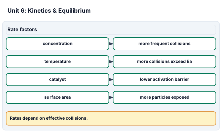
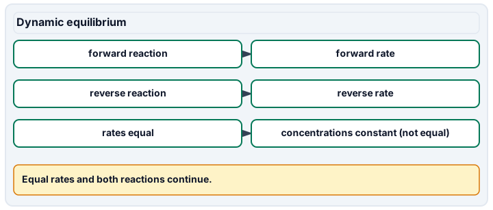
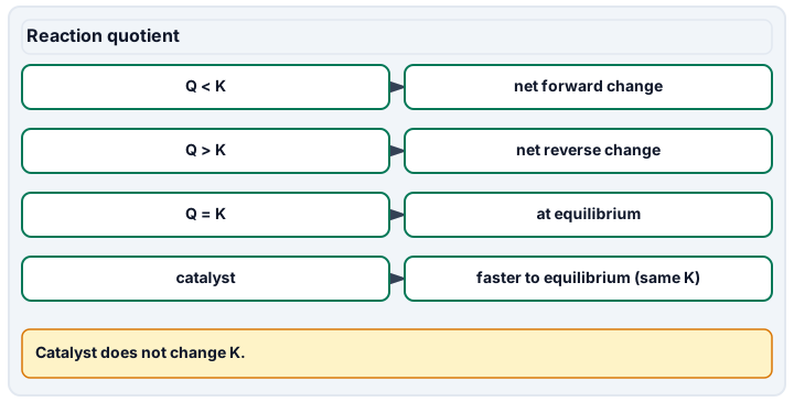
Diagram description
Rate factors maps concentration, temperature, catalyst and surface area to collision or activation-barrier effects. Dynamic equilibrium states forward and reverse rates and equal rates with constant but not equal concentrations. Reaction quotient compares Q to K and states the catalyst effect.
Data, provenance, and assumptions
| Time (s) | A concentration (mol L^-1) |
|---|---|
| 0 | 0.1 |
| 50 | 0.06065306597126335 |
| 100 | 0.036787944117144235 |
| 150 | 0.022313016014842982 |
| Temperature (K) | k (s^-1) |
|---|---|
| 300 | 0.01 |
| 330 | 0.04 |
| kf | kr | ks | NO concentration | O2 concentration |
|---|---|---|---|---|
| 0.4 | 0.2 | 0.5 | 0.1 | 0.2 |
| State | Uncatalyzed energy | Catalyzed energy |
|---|---|---|
| reactants | 0 | 0 |
| transition 1 | 60 | 40 |
| intermediate | 20 | 20 |
| transition 2 | 85 | 65 |
| products | -10 | -10 |
| State | Initial N2O4 (mol L^-1) | Kc |
|---|---|---|
| initial closed system | 0.2 | 0.4 |
| Intervention | Immediate implication |
|---|---|
| halve volume | double both concentrations before reaction |
| add inert gas at constant volume | reacting concentrations unchanged |
| add catalyst | faster equilibration; same Kc |
| raise temperature, forward endothermic | new Kc; needs thermal information |
Paper investigation sequence and exact evidence record
Scope and safety: All new cases are paper/data investigations, not laboratory procedures. Any physical exercise requires prior educator and safety approval, an approved protocol, suitable facilities and accessibility provisions. Do not improvise acid/base, electrolysis, gas, high-voltage, combustion, toxic-substance or unknown-substance experiments from these tables. Supplied records do not demonstrate hands-on technique or performed lab hours.
Materials and preparation
- [kinetic-time] Use kinetic-time, arrhenius-pair and the explicitly different transfer law; retain existing rate-practice as a separate prerequisite.
- [mechanism-energy] Use mechanism-energy and reaction-profile with both stated algebraic hypotheses; all NO labels are symbolic inputs, not substances to obtain.
- [equilibrium-response] Use equilibrium-response and equilibrium-interventions with a paper ICE table; no gas production, compression or handling is assigned.
Procedure and schedule
- [kinetic-time] Question: Which time law is consistent with the given depletion pattern, and which extra records would be needed to test its limitations? Prerequisites: Concentration, rate versus amount, logarithms, inverse concentration and Kelvin/J/kJ conventions.
- [kinetic-time] Design: Time varies within the first model; temperature varies only in the separate k pair. Concentration and apparent k are responses. Controls: Hold volume, initial state and other-reactant/catalyst status fixed within each model; do not pool the distinct datasets. Replication: Exact supplied points are not replicates. A proposed real study would require independent runs and background controls under a separately approved procedure.
- [kinetic-time] Analysis procedure: Compute ratios and transformed slopes, predict held-out points, calculate Ea and list residual patterns that would undermine the model. Record: Retain raw/transformed data with axes and units, k/half-life/Ea chains, fit limitations, proposed replicate design, source/date and the second-order transfer.
- [mechanism-energy] Question: How large is the error from eliminating an intermediate before checking the competing removal timescales? Prerequisites: Elementary versus overall reaction, rate-constant units, intermediates, reversible rates and reading energy profiles.
- [mechanism-energy] Design: Vary the reverse loss constant in the transfer and compare predicted intermediate concentration/rate under two hypotheses. Controls: Keep forward/slow constants, starting concentrations and reaction direction fixed; maintain unchanged thermodynamic endpoints in the profile. Replication: Compare independent derivations and a proposed simulated timescale sweep; supplied single records do not validate a mechanism.
- [mechanism-energy] Analysis procedure: Cancel steps, derive pre-equilibrium and quasi-steady expressions, compare loss rates and relative errors, then calculate local barriers. Record: Keep the elementary steps, units, two predictions, competing loss ratio, error denominator, energy diagram, assumption verdict, source/date and transfer.
- [equilibrium-response] Question: How does a volume perturbation change an equilibrium composition while preserving the same temperature-dependent equilibrium constant? Prerequisites: Balanced reaction coefficients, concentrations, quadratic roots, closed-system material balance and normalized quotients.
- [equilibrium-response] Design: Volume and initial concentration change in separate scenarios; Qc and final species concentrations are the calculated responses. Controls: Fix temperature, gas-model convention, total species-equivalent amount and catalyst-independent Kc during the compression case. Replication: Check substitution into Kc and atom balance independently; synthetic roots are not observed replicate equilibria.
- [equilibrium-response] Analysis procedure: Distinguish initial, immediate-perturbation and re-equilibrated states; solve the quadratic and check physical bounds/approximation size. Record: Retain all three state ledgers, volume/temperature conditions, Qc/Kc comparisons, physical-root checks, atom balance, source/date and dilution transfer.
Record: Label every page with case and dataset IDs, selected readiness level, date and source section. Preserve the independent first attempt, units, assumptions, calculations, uncertainty, feedback and transfer. Cite the specific science criterion; do not sign a practical observation that did not occur. The course-map inventory connects every case to these exact records.
Worked model
[kinetic-time] Using the first two time points, k = ln(0.1000/0.06065306597)/50 = 0.0100 s^-1. Half-life is 69.314718 s, and each 50 s interval multiplies concentration by exp(-0.5), not by a constant subtraction. For the independent temperature pair, ln(k2/k1) = (Ea/R)(1/T1 - 1/T2); Ea = R ln(4)/(1/300 - 1/330) = 38036.765722 J mol^-1 = 38.036766 kJ mol^-1. Do not insert 27 and 57 degrees C into the reciprocals. [mechanism-energy] The pre-equilibrium hypothesis gives [I] = 0.4(0.100)^2/0.2 = 0.0200 M and r = 0.5(0.0200)(0.200) = 0.00200 M s^-1. But the competing loss ratio is 0.100/0.200 = 0.5, not much less than one. Under the alternative quasi-steady hypothesis, [I] = 0.004/0.300 = 0.0133333 M and r = 0.00133333 M s^-1; the pre-equilibrium prediction is 50% larger. The catalyzed second forward barrier is 65 - 20 = 45 kJ mol^-1, and the endpoint ΔH is -10 kJ mol^-1 on both paths. [equilibrium-response] Let x dissociate from 0.200 M. Then [N2O4] = 0.200 - x and [NO2] = 2x; 4x^2/(0.200 - x) = 0.400 gives x = 0.100 M, so equilibrium concentrations are 0.100 and 0.200 M. After instant volume halving they are 0.200 and 0.400 M, with Qc = 0.800 > 0.400, so some NO2 combines. With the new total N2O4-equivalent concentration 0.400 M, solving again gives [NO2] = 0.312310563 M and [N2O4] = 0.243844719 M. The reverse equation has Kc = 2.5; doubling the original equation squares Kc to 0.16.
Numerical calibration
- 0.01 s^-1 for the first-order model
- 69.31471805599 seconds (s)
- 38.03676572215 kJ mol^-1, two-point apparent activation energy
- 0.0333333333333 mol L^-1 in second-order transfer at 100 s
- 0.02 mol L^-1, conditional pre-equilibrium prediction
- 0.002 mol L^-1 s^-1, conditional pre-equilibrium prediction
- 45 kJ mol^-1 from intermediate to transition 2
- 0.001 mol L^-1 s^-1, revised conditional prediction
- 0.2 mol L^-1 NO2 before compression
- 0.1 mol L^-1 N2O4 before compression
- 0.8 dimensionless Qc immediately after compression
- 0.312310562562 mol L^-1 NO2 at new equilibrium
- 2.5 dimensionless Kc for reversed equation
- 0.073205080757 mol L^-1 NO2 from 0.0500 M starting N2O4
Attempt the assigned level
Try the tasks before reading the calibration. These are practice answers, not a secure examination; use a new dataset or changed assumption for the assessed transfer.
Foundation
- [kinetic-time] Read the first-order subsection of Integrated Rate Laws, compare the concentration ratios for equal 50 s intervals and use the supplied log form to compute k with units. State why constant ratios differ from constant concentration losses.
- [mechanism-energy] Use Reaction Mechanisms to cancel I from the steps and distinguish intermediate from catalyst. From reaction-profile, calculate catalyzed second-step barrier and reaction enthalpy without using the zero of the graph as the start of every step.
- [equilibrium-response] From Equilibrium Constants, write Qc and distinguish equal rates from equal concentrations. Verify the worked equilibrium against Kc and conserved amount, then judge whether a very large K would prove rapid or complete conversion.
Check after your attempt
- [kinetic-time] Each interval retains exp(-0.5), about 0.60653, of the previous concentration, so absolute losses shrink. k = 0.0100 s^-1 and half-life 69.314718 s. A zero-order model instead subtracts a constant amount per equal time interval until its assumptions fail.
- [mechanism-energy] I is produced in step one and consumed in step two; it cancels from 2NO + O2 -> 2NO2. A catalyst is regenerated rather than a net product. The catalyzed second barrier is 45 kJ mol^-1 from the intermediate at 20 to the peak at 65; endpoint ΔH stays -10 kJ mol^-1.
- [equilibrium-response] Qc is normalized NO2 squared divided by normalized N2O4. Equal nonzero opposing rates do not require equal amounts. With 0.200 M NO2 and 0.100 M N2O4, Qc = 0.400 and [N2O4] + [NO2]/2 = 0.200 M. Even a large K describes a coefficient-weighted equilibrium tendency, not a rate or a guarantee that no reactant remains.
High-school core: typically grades 9-10
- [kinetic-time] Calculate half-life and check the 100/150 s concentrations from the law rather than copying them. Use Collision Theory to derive the two-temperature Ea and explain the J-versus-kJ choice for R.
- [mechanism-energy] Derive the conditional pre-equilibrium [I] and rate from the supplied constants, with units. Compare kr to ks[O2] and decide whether the numerical record actually supports the approximation.
- [equilibrium-response] Use Equilibrium Calculations to solve the initial ICE table, then calculate immediate Qc and the new equilibrium after halving volume. Reject the nonphysical root and test the small-x approximation instead of merely asserting a shift.
Check after your attempt
- [kinetic-time] Half-life is 69.314718 s; predicted [A] at 100 and 150 s is 0.0367879441 and 0.0223130160 M. The Arrhenius pair gives 38.036766 kJ mol^-1 after calculating in joules with R = 8.314462618 J mol^-1 K^-1. Mixing kJ in Ea with a joule-based R would introduce a factor-of-1000 error.
- [mechanism-energy] The hypothesis gives [I] = 0.0200 M and r = 0.00200 M s^-1. kf/kr has units L mol^-1, so multiplying by [NO]^2 gives M. kr is 0.200 s^-1 and ks[O2] 0.100 s^-1, so consumption is not negligible relative to reversal; pre-equilibrium is not established.
- [equilibrium-response] The positive physical initial x is 0.100 M; a negative extent contradicts starting without NO2. Compression makes Qc = 0.800 and forces reverse change to [NO2] = 0.312310563 M. Initial x is half the starting N2O4, so ignoring depletion would be a large error rather than a valid small-change approximation.
Honors extension: typically grades 11-12
- [kinetic-time] Design a residual/replicate check to distinguish first-order behavior from alternative laws and explain why a two-point Arrhenius fit is not mechanism validation. Contrast first-order and second-order half-life dependence on initial concentration.
- [mechanism-energy] Compute the alternative quasi-steady prediction and its relative difference from pre-equilibrium. Specify a timescale/composition test before trusting either approximation and explain why unchanged endpoints do not mean unchanged activation barriers.
- [equilibrium-response] Use Shifting Equilibria to compare constant-volume inert-gas addition, a catalyst and heating of this endothermic forward reaction. Derive the reversed/doubled Kc values and explain why concentration-standard Kc must not silently replace pressure-standard Kp in a Gibbs calculation.
Check after your attempt
- [kinetic-time] Inspect residuals for [A], ln[A] and 1/[A] models across several times with independent preparations and background controls; do not prefer a transform only because two points align. More temperatures are needed to inspect curvature. First-order half-life is independent of [A]0; for rate k[A]^2 it is 1/(k[A]0), so dilution lengthens it.
- [mechanism-energy] Quasi-steady [I] is 0.0133333 M and r 0.00133333 M s^-1; the pre-equilibrium rate is 50% higher relative to that value. Resolve the model intermediate relaxation time against reactant depletion and vary model [O2] in a simulation. A catalyst can lower both-direction barriers while preserving endpoint ΔH and thermodynamic K.
- [equilibrium-response] Inert gas at constant volume leaves reacting concentrations/Qc unchanged; catalyst leaves Kc unchanged. Heating this endothermic forward reaction increases Kc. Reversal gives 2.5 and doubled stoichiometry 0.16. Because Δn(gas) is +1, pressure and concentration normalization differ by an RT/reference factor, so standard-state consistency must be checked before using -RT ln K.
History, reading, and writing connection
Extend the existing source-linked catalyst discussion by comparing the assigned kinetic and equilibrium models. Explain how “faster” and “greater equilibrium yield” led to different constraints in an industrial process; cite the actual section and state a limitation rather than inventing operating conditions.
Write in your own words or use an approved accessible equivalent. Cite a specific assigned section or figure, identify its evidence, and state one limitation or counterargument. Use the AI practice contract only for permitted coaching, never to invent observations or write the assessed response.
Transfer to a new case
[kinetic-time] For a distinct second-order model rate = k[A]^2 with k = 0.200 L mol^-1 s^-1 and [A]0 = 0.100 M, calculate [A] after 100 s. Decide whether the prior exponential or fixed half-life can be reused. [mechanism-energy] Double kr to 0.400 s^-1 and keep all other mechanism-energy inputs fixed. Calculate the revised conditional pre-equilibrium rate and determine whether a factor-four reverse-to-consumption timescale separation is conclusive validation. [equilibrium-response] Use the same 298 K Kc but begin with only 0.0500 M N2O4 in a new closed model vessel. Solve for equilibrium NO2, verify the material balance, and judge whether the initial dissociated fraction stays the same after dilution.
Calibration: [kinetic-time] 1/[A]100 = 1/0.100 + 0.200(100) = 30 L mol^-1, so [A]100 = 0.033333333 M. The exponential is not the specified law, and successive second-order half-lives lengthen as concentration decreases; the previous fixed first-order half-life is inapplicable. [mechanism-energy] The conditional intermediate halves to 0.0100 M and r becomes 0.00100 M s^-1. The loss ratio is now 0.100/0.400 = 0.25, still not clearly negligible; the quasi-steady value would be 0.000800 M s^-1. A smaller discrepancy is not proof that pre-equilibrium is valid. [equilibrium-response] 4x^2/(0.0500 - x) = 0.400 gives x = 0.036602540 M and NO2 = 0.073205081 M. N2O4 is 0.013397460 M, and 0.013397460 + 0.073205081/2 = 0.0500 M. The dissociated fraction is larger than one half, so K constant does not mean constant percent conversion.
Evidence to retain
[kinetic-time] Criteria 1–2: keep initial-rate work already assigned, then add time-law selection, dimensional k, half-life, Arrhenius energy and a qualified fit inference. Criterion 5 receives analysis planning only; the constructed curve is not evidence of measuring a reaction rate. [mechanism-energy] Science criteria 1–3: retain elementary-step cancellation, rate-law derivation with dimensions, the failed-approximation comparison and energy-profile barriers. These supplement existing rate-practice; do not claim a kinetic fit establishes causation, mechanism uniqueness or a changed equilibrium constant. [equilibrium-response] Criteria 3–4: retain Q/K expressions with state conventions, ICE table, root selection, material balance and quantitative perturbation. Criterion 5 receives prediction/analysis evidence but a supplied gas calculation is not a performed equilibrium-shift or rate observation.
Record units, calculations, source/date, uncertainty, and what is measured versus inferred. A simulation or supplied dataset must stay labeled as such. All new cases are paper/data investigations, not laboratory procedures. Any physical exercise requires prior educator and safety approval, an approved protocol, suitable facilities and accessibility provisions. Do not improvise acid/base, electrolysis, gas, high-voltage, combustion, toxic-substance or unknown-substance experiments from these tables. Supplied records do not demonstrate hands-on technique or performed lab hours.
Return to all eight learning pathways. Print this unit page for the student lessons; the linked five-page packet remains the separate assessment companion.
Unit mastery rubric
| Criterion | Developing | Proficient | Mastery |
|---|---|---|---|
| Reaction rate & factors | Cannot explain rate changes or compare initial rates. | Explains factors or rate ratios but needs help deriving the law, units, or prediction. | Explains concentration, temperature, surface-area and catalyst effects; derives orders from initial-rate comparisons (not equation coefficients), calculates k with units, and predicts a new rate. |
| Kinetic models & activation energy | Thinks every collision yields a reaction. | Uses a kinetic formula but needs help choosing a law, barrier or approximation. | Uses collision theory and energy profiles; checks integrated rate laws, Arrhenius units and mechanism approximations without treating a fit as unique mechanistic proof. |
| Dynamic equilibrium | Believes reactions simply stop at equilibrium. | Says rates are equal but calls the system static. | Describes equilibrium as equal forward and reverse rates with constant concentrations. |
| Le Châtelier's principle & K | Cannot predict the effect of a stress. | Predicts a shift's direction but not its cause or the role of K. | Predicts shifts from concentration, temperature or pressure; compares Q with K, solves equilibrium material balances, checks approximations, and distinguishes catalyst effects from changes in K. |
| Lab technique (rate / equilibrium shift) | Cannot observe or time a rate change. | Collects data but draws conclusions loosely. | Measures a rate or induces a visible equilibrium shift and links the observation to theory. |
| Integration (cross-domain) | Makes no supported connection between the source and the science. | Uses the source but needs help connecting evidence, writing, or limitations to the science. | Independently connects History, Reading, and Writing using a cited source, appropriate evidence, a limitation, and a scientific explanation. |
Integration is reported separately and cannot lower the science grade or block a science demonstration pass. Science and practical criteria determine that pass. Use the integration guide's evidence checklist for the separately reported criterion.
“A catalyst speeds both forward and reverse reactions but does not shift the equilibrium position or change K. Adding product does shift the equilibrium toward reactants. Rate and equilibrium yield are different questions.”
“Hotter just means faster. Equilibrium means both sides are equal amounts, I think.”
Complete the assigned rate-law calculation and fresh transfer, then retain the rate investigation and equilibrium-shift demonstration under an instructor-approved, supervised procedure. A named chemical example is never permission to handle reagents. Judge each science criterion from its own evidence; the calculations do not substitute for criterion 5's practical work. Explain each approved observation with theory, and keep predictions, synthetic data, and actual observations distinct.
A 5-page clipboard packet — unit overview, key terms, the mastery rubric, anchor examples, and a score sheet you can print and grade against.