Unit 06 · Climate & Climate Change
This unit separates the weather outside the window from the climate of a place over decades. It covers what sets a region's climate zone, how the greenhouse effect keeps the planet warm and what happens when its balance shifts, how scientists read past climate from proxies — ice cores, tree rings, sediment — and how carbon moves through ocean, air, rock, and life in the carbon cycle. Mastery means you can tell weather from climate and read a proxy record as evidence of change over time, not a single day's forecast.
Student learning: Test natural and human explanations for climate change against measured records
Choose the level by readiness, not age alone, and record it before instruction. Foundation, core, and honors tasks are study pathways, not an AP course or a promise of college credit. The instructor retains practical assessment and the published science rubric; integration is reported separately.
Prerequisites: Foundation: means, signed differences, unit conversion and graph axes. Core: elapsed-year rates, baselines, linear calibration and monthly running totals. Honors: least-squares slope, residuals and baseline shifts. Readiness check: an annual mean of 13.8 C minus a 14.0 C baseline is -0.2 C, and 4 C over 5,000 years is 4/5000 x 100 = 0.08 C per century. Practice both before trend fitting.
Suggested sequence: read and discuss the explanation; attempt the worked model; analyze the data at your selected level; check the answers; then complete the source-linked response and a fresh transfer question. These activities supplement, not replace, supervised practical work and the full-year schedule.
Assigned reading and focus
- NOAA Global Monitoring Laboratory: Mauna Loa annual mean CO2 data. Read the file header and the 1960, 1980, 2000 and 2020 rows. Cite NOAA GML and the Scripps Institution of Oceanography record credited in the header. The frozen excerpt below comes from the file created 2026-09-05, accessed 2026-09-27.
- NOAA Climate.gov: Climate Change, Global Temperature. Read Why global surface temperature matters and Past and future change in global temperature, including the quoted IPCC ranges for each contributor to warming. Record the reported rates of 0.06 C per decade since 1850 and 0.20 C per decade since 1975. Use the independent synthetic temperatures below for anomaly arithmetic; do not label them as NOAA global observations. Checked 2026-10-02.
- NOAA NCEI: What Are Proxy Data?. Read the introduction and Ice Cores section. Distinguish a measured proxy characteristic, a temperature reconstruction and gases trapped in bubbles; ice age and gas age can differ.
- NASA Earth Observatory: Global Warming. Read the opening paragraph and the paragraphs on how today's warming compares with past warming and on natural causes before the Industrial Revolution. Record the 4 to 7 C rise over about 5,000 years as Earth moved out of ice ages, and the natural drivers named: wobbles in Earth's orbit, changes in the Sun and volcanic eruptions. The article was first written in 2010, so take current rates from NOAA. Checked 2026-10-02.
- NASA Science: The Causes of Climate Change. Read Evidence Shows That Current Global Warming Cannot Be Explained by Solar Irradiance. List each line of evidence and the prediction it tests, including what a more active Sun would do to the upper atmosphere. Checked 2026-10-02.
- USGS Volcano Hazards Program: Volcanoes Can Affect Climate. Read Sulfate aerosols can cool the climate and the section asking whether volcanoes emit more CO2 than human activities. Note the one-to-three-year cooling after large eruptions and the statement that present-day volcanoes release less than 1 percent of the CO2 released by human activities. Checked 2026-10-02.
- USGS Water Science School: Snowmelt Runoff and the Water Cycle. Read the opening section and Contribution of snowmelt to streamflow. Note how mountain snowpack works as a natural reservoir in the western United States and the statement that as much as 75 percent of water supplies in some western states come from snowmelt. Checked 2026-10-02.
Learn the science
Earth's climate has always changed. NASA explains that before the Industrial Revolution, climate changed mostly because of variations in sunlight, including tiny wobbles in Earth's orbit and changes in the Sun itself, while large volcanic eruptions cooled the planet for a time. As Earth moved out of ice ages, global temperature rose about 4 to 7 C over roughly 5,000 years. People who disagree about today's causes can start from this shared record: climate changes naturally, and Earth has warmed since the last ice age.
The open questions are how much of recent warming is natural, how much comes from people, and how much more to expect. Treat each candidate as a hypothesis with its own prediction. Continued recovery from the ice age predicts warming near the ice-age pace. A brighter Sun predicts rising solar energy and warming in every layer of the atmosphere. Volcanoes predict brief cooling after large eruptions. Ocean cycles such as El Nino, part of what scientists call internal variability, predict swings up and down rather than a steady climb. Added greenhouse gases predict a warming surface and lower atmosphere while the upper atmosphere cools.
Then check each prediction. NOAA reports global warming of 0.06 C per decade since 1850 and 0.20 C per decade since 1975, far faster than the ice-age average. NASA reports that the Sun's average energy has stayed level or fallen slightly since 1750 while the upper atmosphere has cooled. USGS reports that large eruptions cooled the surface for one to three years and that present-day volcanoes release less than 1 percent of the CO2 that human activities do. The IPCC ranges quoted by NOAA put natural drivers and internal variability within about 0.1 to 0.2 C either way and the human-caused total at 0.8 to 1.3 C. A failed prediction sends an explanation to review; a held one strengthens an explanation without proving it.
The CO2 values are observed annual dry-air mole fractions from one monitoring record, in micromol/mol (ppm), not a globally averaged temperature or an emissions inventory. Only four widely spaced years are supplied; these do not describe seasonal variation or all interannual behavior.
The reported 0.12 ppm uncertainty is the file's estimated annual-mean uncertainty based on differences between independently determined NOAA and Scripps annual means. It is not a confidence interval for a regression or a measure of spatial representativeness.
An anomaly subtracts a stated baseline. The separate temperature table is wholly synthetic and uses an invented 1961-1990 site baseline of 14.0 C. Changing that baseline shifts every anomaly by the same amount but does not change a slope.
For least-squares y = a + bx, b = sum((x - mean(x))(y - mean(y)))/sum((x - mean(x))^2), a = mean(y) - b mean(x). A residual is observed minus fitted y. Use x = years since 1960 to avoid a large intercept; convert C/year to C/decade by multiplying by 10.
A trend or correlation is not causal proof. NOAA and NASA conclude from physical mechanisms and several independent lines of evidence that human-produced greenhouse gases are the main cause of recent warming; fitting four CO2 points or pairing them with an invented temperature record cannot establish that on its own. Scientists still give ranges rather than single numbers for the human share and for how much more warming to expect, and families disagree about the size of the human share and about what policy, if any, should follow. This unit does not take a policy position. Do not infer climate sensitivity from these tables.
For the synthetic ice example only, temperature anomaly = 2 x (isotope value + 35) C. This is an assigned local linear calibration, not a universal isotope thermometer. Age, moisture source, seasonality and calibration uncertainty can alter a reconstruction; gas in bubbles need not have the same age as the surrounding ice.
Whatever the cause of a warm, dry year, farms, ranches and towns still have to plan for water. USGS describes mountain snowpack as a natural reservoir for the western United States and notes that some western states draw as much as 75 percent of their water supply from snowmelt. The invented basin below shows why timing matters as much as the total: the same runoff can leave a late-summer shortage when it arrives before irrigation season. Storage, efficient irrigation and conservation make sense under any explanation of the cause.

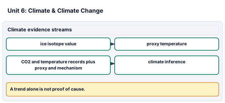
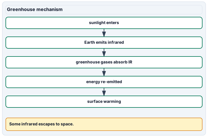
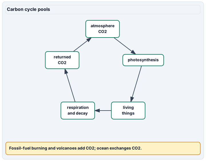
Diagram description
The ice-isotope value becomes a proxy temperature through calibration; observed CO2 and temperature records, the proxy temperature and the physical mechanism are then combined for a climate inference. The greenhouse panel shows sunlight, emitted infrared, greenhouse gas absorption, escaping infrared, re-emission and warming. The carbon cycle shows atmospheric CO2 taken up by photosynthesis into living things and returned by respiration and decay as CO2; the caption adds that fossil-fuel burning and volcanoes add CO2 and that the ocean absorbs and releases CO2.
Data, provenance, and assumptions
| Year | Annual mean CO2 (ppm) | Reported annual-mean uncertainty (ppm) |
|---|---|---|
| 1960 | 316.91 | 0.12 |
| 1980 | 338.76 | 0.12 |
| 2000 | 369.71 | 0.12 |
| 2020 | 414.21 | 0.12 |
| Year | Synthetic annual mean (C) | Synthetic baseline mean (C) |
|---|---|---|
| 1960 | 13.8 | 14 |
| 1980 | 14 | 14 |
| 2000 | 14.5 | 14 |
| 2020 | 14.7 | 14 |
| Ice age (years BP) | Isotope value (per mil) |
|---|---|
| 0 | -35 |
| 10000 | -38 |
| 20000 | -40 |
| Record | Temperature change (C) | Time span (years) | Source |
|---|---|---|---|
| Out of past ice ages, low estimate | 4 | 5000 | NASA Earth Observatory |
| Out of past ice ages, high estimate | 7 | 5000 | NASA Earth Observatory |
| Global average since 1850 | 0.06 | 10 | NOAA Climate.gov |
| Global average since 1975 | 0.2 | 10 | NOAA Climate.gov |
| Contributor | Low (C) | High (C) |
|---|---|---|
| Total human-caused (best estimate 1.07 C) | 0.8 | 1.3 |
| Well-mixed greenhouse gases | 1 | 2 |
| Other human drivers, mainly aerosols | -0.8 | 0 |
| Natural drivers: solar and volcanic | -0.1 | 0.1 |
| Internal variability | -0.2 | 0.2 |
| Month | Cooler-spring runoff (million m^3) | Warmer-spring runoff (million m^3) | Farm and town demand (million m^3) |
|---|---|---|---|
| April | 10 | 20 | 5 |
| May | 25 | 40 | 10 |
| June | 35 | 25 | 15 |
| July | 20 | 10 | 30 |
| August | 10 | 5 | 30 |
| September | 0 | 0 | 10 |
Worked model
Observed CO2 rises 414.21 - 316.91 = 97.30 ppm over 60 years: the endpoint-average rate is 1.6217 ppm/year. The separate synthetic anomalies are -0.2, 0, 0.5 and 0.7 C. Their endpoint rate is 0.9/60 x 10 = 0.15 C/decade. To compare a modern rate with the ice-age record, put both in the same units: 4 C over 5,000 years is 4/5000 x 100 = 0.08 C per century. These are different variables with different provenance; equal calendar labels do not create a causal experiment.
Numerical calibration
- 1.6217 ppm/year, observed endpoint average
- 1.61425 ppm/year, four-point least-squares slope
- -0.2 C relative to the synthetic 14.0 C baseline
- 0.16 C/decade, synthetic four-point fit
- -10 C under the assigned proxy calibration only
- 0.08 C per century, NASA low ice-age estimate
- 0.14 C per century, NASA high ice-age estimate
- 0.6 C per century, NOAA rate since 1850
- 2 C per century, NOAA rate since 1975
- 25 times the low ice-age average, for the rate since 1975
- 0.3 C, upper bound for natural drivers plus internal variability in the quoted ranges
- 55 million m^3 April-June surplus in the warmer spring
- 10 million m^3 September shortage with 45 million m^3 of storage
- 4 million m^3 shortage after a 10 percent July-August demand cut
- 14.285714 % of July-September demand needed to remove the warmer-spring shortage
Attempt the assigned level
Try the tasks before reading the calibration. These are practice answers, not a secure examination; use a new dataset or changed assumption for the assessed transfer.
Foundation: typically grades 7-8
- Calculate all four synthetic anomalies and draw labeled year/anomaly axes. State the baseline and why a negative anomaly does not mean a negative Celsius temperature. Then calculate the observed CO2 change from 1960 to 2020 in ppm and percent of the 1960 value, labeling the CO2 dataset observed and the temperature dataset synthetic.
- Convert both NASA ice-age figures and both NOAA rates to C per century. Order the four rates and name the explanation for recent warming that this comparison tests.
- For each month in the invented basin, subtract demand from runoff in both springs. Find each spring's April-June surplus and explain why the warmer spring can run short in late summer even though its total runoff is the same.
Check after your attempt
- Anomalies are -0.2, 0, 0.5 and 0.7 C relative to the invented 14.0 C baseline; 13.8 C is positive even though its anomaly is negative. The observed CO2 increase is 97.30 ppm, about 30.7% of 316.91 ppm. A percentage increase in atmospheric mole fraction is not the percentage of Earth's warming caused by CO2.
- Ice-age warming averages 0.08 to 0.14 C per century; NOAA reports 0.6 C per century since 1850 and 2.0 C per century since 1975. The rate since 1850 is about 4.3 to 7.5 times the ice-age average and the rate since 1975 about 14.3 to 25 times. This counts against "still recovering from the ice age at the usual pace" but does not test the Sun, volcanoes or greenhouse gases.
- Cooler spring: +5, +15, +20, -10, -20 and -10, with a 40 million m^3 April-June surplus. Warmer spring: +15, +30, +10, -20, -25 and -10, with a 55 million m^3 surplus. The totals match, but more water arrives before irrigation season and is useful in July-September only if it can be stored.
High-school core: typically grades 9-10
- Calculate CO2 endpoint rates over 1960-1980 and 2000-2020 and compare them with the full-span rate without claiming a constant future rate. Then apply the supplied ice calibration to all three proxy rows, give the oldest row's temperature sensitivity to +/-0.2 per mil, and explain why this is a proxy reconstruction, not a thermometer record.
- Build a competing-explanations table for recent warming with five rows: recovery from the ice age, a brighter Sun, volcanoes, ocean cycles and added greenhouse gases. For each, write its prediction, the evidence from the assigned readings or the attribution table, and whether the prediction held.
- Usable storage in the invented basin is 45 million m^3 and starts empty on April 1. Find the July-September shortage in each spring, then recalculate the warmer spring after farms and town cut July and August demand by 10 percent.
Check after your attempt
- Early rate: (338.76 - 316.91)/20 = 1.0925 ppm/year. Late rate: (414.21 - 369.71)/20 = 2.225 ppm/year. The full-span 1.6217 lies between them and is not a forecast. Model proxy anomalies are 0, -6 and -10 C; the oldest row has +/-0.4 C sensitivity from isotope error alone. It remains a calibrated inference with unquantified dating and calibration errors, not a direct temperature measurement.
- Ice-age recovery predicts 0.08-0.14 C per century; NOAA's rates are far higher, so it fails as a full explanation. A brighter Sun predicts rising solar energy and warming in every layer; NASA reports level or slightly lower solar energy and a cooling upper atmosphere. Volcanoes predict brief cooling, which USGS confirms, and their CO2 is under 1 percent of human emissions. Ocean cycles predict swings, and the quoted range for internal variability is -0.2 to +0.2 C. Greenhouse gases predict surface warming with upper-atmosphere cooling, which matches. A held prediction strengthens an explanation without proving it.
- Cooler spring: the 40 million m^3 surplus all fits in storage and covers the 40 million m^3 summer deficit, so there is no shortage. Warmer spring: storage is full at the end of May, so 10 of the 55 surplus passes downstream, and summer needs 55, leaving a 10 million m^3 shortage in September. The 10 percent cut saves 6, so the shortage falls to 4 million m^3. The plan works whatever caused the warm spring.
Honors extension: typically grades 11-12
- Fit lines to the four observed CO2 means and, separately, the four synthetic temperature anomalies using years since 1960. Report slopes, temperature residuals and the difference from endpoint slopes.
- Change the synthetic baseline from 14.0 to 14.2 C and recompute anomalies. Bound its 1960-2020 endpoint trend using +/-0.1 C at each endpoint. Explain why neither a fit nor this bound establishes causal attribution.
- The NASA ice-age figure averages proxy records over about 5,000 years, while the NOAA rates come from thermometer records over decades. Explain one way this comparison could mislead, and what evidence would make it fairer. Then use the attribution table to find the largest warming that natural drivers and internal variability together could contribute.
- With 45 million m^3 of storage, what percentage cut in total July-September demand would remove the warmer-spring shortage? Name one way farms and one way the town could reach it, and one cost each choice carries.
Check after your attempt
- CO2 least-squares slope = 1.61425 ppm/year with intercept 311.47 ppm at x = 0; synthetic temperature slope = 0.016 C/year = 0.16 C/decade, intercept -0.23 C. Temperature residuals are 0.03, -0.09, 0.09 and -0.03 C. Fits use all four points; endpoint rates are 1.6217 ppm/year and 0.15 C/decade.
- New anomalies: -0.4, -0.2, 0.3 and 0.5 C; slope remains 0.16 C/decade. Endpoint differences span 0.7-1.1 C over 60 years, or 0.1167-0.1833 C/decade. This is a sensitivity interval, not a fitted-slope confidence interval or causal proof.
- A long average can hide faster and slower intervals, and proxies can smooth out short changes, so a brief rapid warming in the past might not show. A fairer test compares rates over matched time spans, using records with enough time resolution and several independent reconstructions. The upper ends of the natural and internal-variability ranges add to 0.1 + 0.2 = 0.3 C, below the 0.8 C low end of the human-caused range; the ranges are separate assessments, so this is a bound, not an exact sum.
- July-September demand is 70 million m^3 and the shortage is 10, so a 10/70 = 14.29 percent cut is needed. Farms might switch some fields to more efficient irrigation or adjust crop timing; the town might limit summer lawn watering. Each choice costs money, yield or convenience, and the people affected should weigh it.
History, reading, and writing connection
Using the NOAA file header, the NCEI proxy explanation and the NASA and USGS readings, write a one-page evidence brief on one question: what do these sources say caused recent warming, and how did they test the alternatives? Name at least three explanations, give the prediction each makes and the evidence that supports or fails it, and say which numbers were observed, which were reconstructed from proxies and which were invented. Report what NOAA and NASA conclude and one limitation of the evidence, and keep any opinion about policy out of the science section.
Write in your own words or use an approved accessible equivalent. Cite a specific assigned section or figure, identify its evidence, and state one limitation or counterargument. Use the AI practice contract only for permitted coaching, never to invent observations or write the assessed response.
Transfer to a new case
A new fictional site has means 12.0 C in 1980 and 12.6 C in 2010, relative to an assigned 11.8 C baseline. Foundation: find anomalies. Core: find the endpoint trend. Honors: add 0.3 C to the baseline and test whether the slope changes. All levels: distinguish these synthetic quantities from causal evidence.
Calibration: Foundation: anomalies are 0.2 and 0.8 C. Core: the endpoint trend is 0.6/30 x 10 = 0.2 C/decade. Honors: a 12.1 C baseline gives -0.1 and 0.5 C, with the same slope. Neither baseline choice nor this two-point synthetic trend proves a cause.
Evidence to retain
At the agreed level retain the provenance-labeled graphs, baseline/interval work, selected fit or proxy calculation, the rate comparison and competing-explanations table, the basin water budget and the new-site transfer. Assess the Climate quantities and Record and proxy reasoning science criteria; use historical/source writing for separately reported integration. No field data collection is assigned. NOAA GML and NCEI sources checked 2026-09-27; NOAA Climate.gov, NASA and USGS sources checked 2026-10-02.
Record units, calculations, source/date, uncertainty, and what is measured versus inferred. A simulation or supplied dataset must stay labeled as such. No field exposure or weather chasing; no water sampling, ingestion, or chemical tests; no solar viewing. Use supplied data and approved images or non-destructive indoor alternatives only. A worksheet does not demonstrate practical performance or authorize a real location or safety forecast.
Return to all eight learning pathways. Print this unit page for the student lessons; the linked five-page packet remains the separate assessment companion.
Unit mastery rubric
| Criterion | Developing | Proficient | Mastery |
|---|---|---|---|
| Climate quantities | Confuses an anomaly, baseline, rate or weather event. | Calculates with help but omits the time span or provenance. | At the agreed level, defends anomalies, endpoint rates or fitted slopes/residuals with baselines, units and limits. |
| Climate zones & what sets them | Cannot say why one place is a desert and another a rainforest. | Names climate zones but not the factors — latitude, altitude, currents — that set them. | Explains how latitude, elevation, ocean currents, and winds combine to set a region's climate zone. |
| Greenhouse effect & the carbon cycle | Thinks the greenhouse effect is only harmful, or confuses it with the ozone hole. | Describes the greenhouse effect but cannot trace carbon through its reservoirs. | Explains how greenhouse gases trap heat and traces carbon through ocean, atmosphere, rock, and life. |
| Record and proxy reasoning | Calls invented temperatures observations or trends causal proof. | Labels sources but needs help explaining a proxy calibration. | At the agreed level, distinguishes observed CO2, synthetic temperatures and proxy inference, with uncertainty and a causal limitation. |
| Climate-data method | Omits axes, source or baseline. | Labels the graph but cannot explain a changed baseline. | Defends the fresh site transfer and retains source/version, baseline and units; does not infer climate sensitivity from these tables. |
| Integration (cross-domain) | Makes no supported connection between the source and the science. | Uses the source but needs help connecting evidence, writing, or limitations to the science. | Independently connects History, Reading, and Writing using a cited source, appropriate evidence, a limitation, and a scientific explanation. |
Integration is reported separately and cannot lower the science grade or block a science demonstration pass. Science and practical criteria determine that pass. Use the integration guide's evidence checklist for the separately reported criterion.
“The observed CO2 endpoint rate is about 1.622 ppm/year. The separate, synthetic temperature fit is 0.16 C/decade; changing its baseline moves the intercept, not that slope. The ice exercise reconstructs a temperature using an assumed calibration. These calculations do not, by themselves, prove a cause of warming.”
“It snowed last week, so global warming can’t be real. Weather and climate are pretty much the same thing anyway.”
At the agreed level, submit source-labeled graphs, baseline/rate or fit/proxy work and the new-site transfer. Distinguish the observed NOAA record from synthetic exercises and trend evidence from causal attribution. These are science criteria; historical/source writing is separately reported integration. No field measurements are required.
A 5-page clipboard packet — unit overview, key terms, the mastery rubric, anchor examples, and a score sheet you can print and grade against.